

In the heliosphere, particles of solar origin (e.g., solar energetic charged particles) and those from our galaxy (galactic cosmic rays, GCRs, i.e., protons, electrons and nuclei with relative abundances drastically dropping above Z=28) dynamically modify their populations (i.e., the space radiation environment) due to the Sun's activity. This latter cyclically passes through low and high periods of activity (e.g., see NOAA space weather prediction center) every about 11 years (these are termed solar or sunspot cycles).
In the following discussion. we will treat a few properties of cosmic rays (CRs) flux expressed as a function of both particle energy and electronic stopping power, i.e., the latter CR distribution is the one used in dealing with single event effects (SEE). The observation data [M. Aguilar et al. (2015)] are those provided by AMS-02 experiment on board of the International Space Station and, for the current case study, the chosen medium is silicon.
The text is organized in sections:
- Cosmic protons from AMS-02 experiment and protons flux fraction corresponding to energy range covered by SRIM data regarding electronic stopping power,
- Modulation effects on protons observed by AMS-02,
- Properties of cosmic rays flux as a function of particle energy or electronic stopping power,
- Impact of employing the restricted energy-loss.
Cosmic Protons from AMS-02 experiment and protons flux fraction corresponding to energy range covered by SRIM data regarding electronic stopping power
The experimental data (Table 1) employed in the current treatment are those provided by AMS-02 and regards the cosmic protons flux (see [M. Aguilar et al. (2015)]). It has to be noted that the AMS-02 data were collected from 19 May 2011 up to 26/11/2013 (i.e., corresponding to a time duration of 79'660'800 seconds).
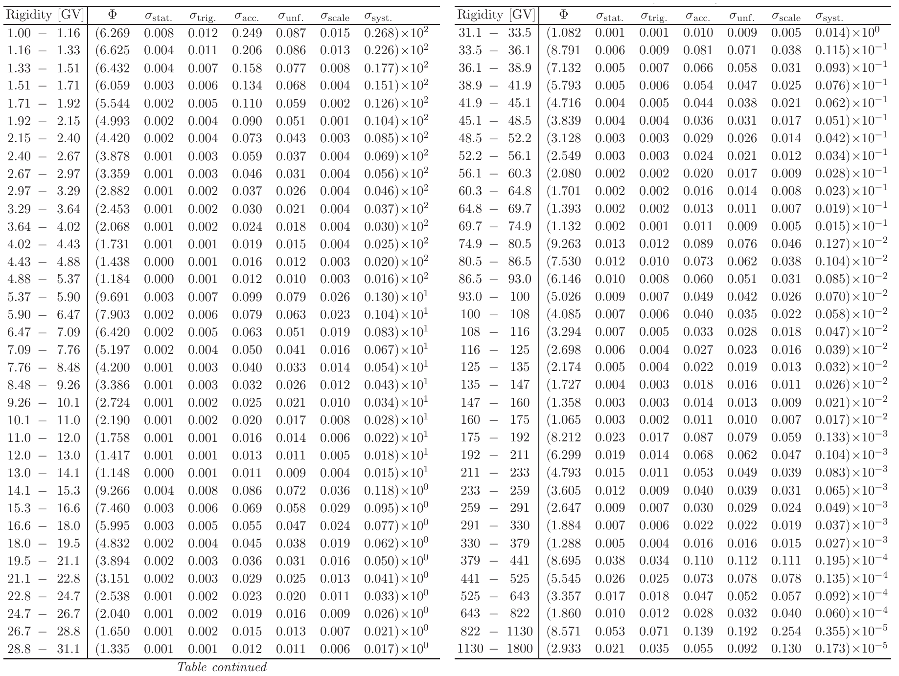
Table 1. The proton flux Φ as a function of rigidity at the top of AMS in units of [m2 · sr · s · GV]−1 including errors due to statistics (stat.); contributions to the systematic error from the trigger (trig.); acceptance, background contamination, geomagnetic cutoff, and event selection (acc.); the rigidity resolution function and unfolding (unf.); and the absolute rigidity scale (scale); and the total systematic error (syst.).From [M. Aguilar et al. (2015)].
The proton fluxes - as used in the current webpage - are those derived from those reported in Table 1 by integrating the flux over the solid angle and transformed as a function of proton kinetic energy and are shown in units of [cm2 · s · MeV]−1. It has to be remarked that one finds that the particle rigidity R is proportional to βγ:
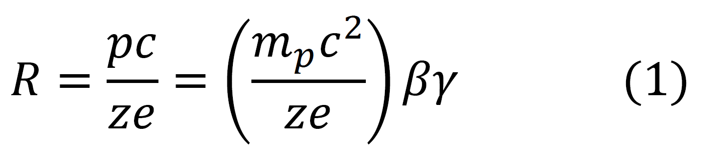 with p the particle momentum, mp the particle rest mass, c the speed of light, z the charge number and, finally, e the electron charge. In Figure 1 the AMS-02 proton flux in units of [cm2 · s · MeV]−1 is shown as function of proton kinetic energy, while in Figure 2 the flux is expressed as a function of βγ [see Eq. (1)].
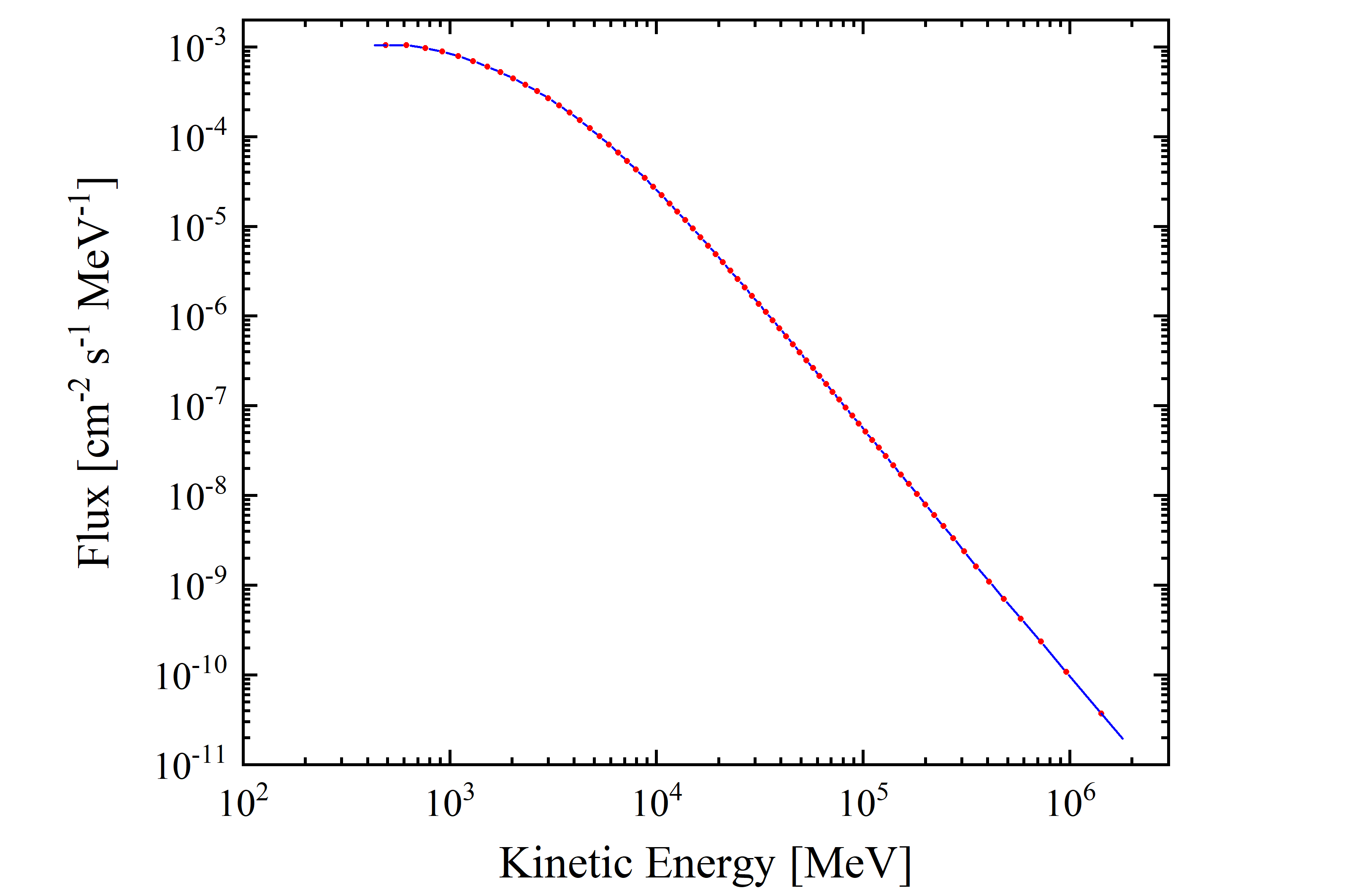
Figure 1. AMS02 proton flux data from [M. Aguilar et al. (2015)] as a function of kinetic energy. Data points (red) are extracted from table 1. The interpolation line (blu) is shown from the lower limit of the first energy bin(433 MeV) to the upper limit of the last one (1.8 TeV).
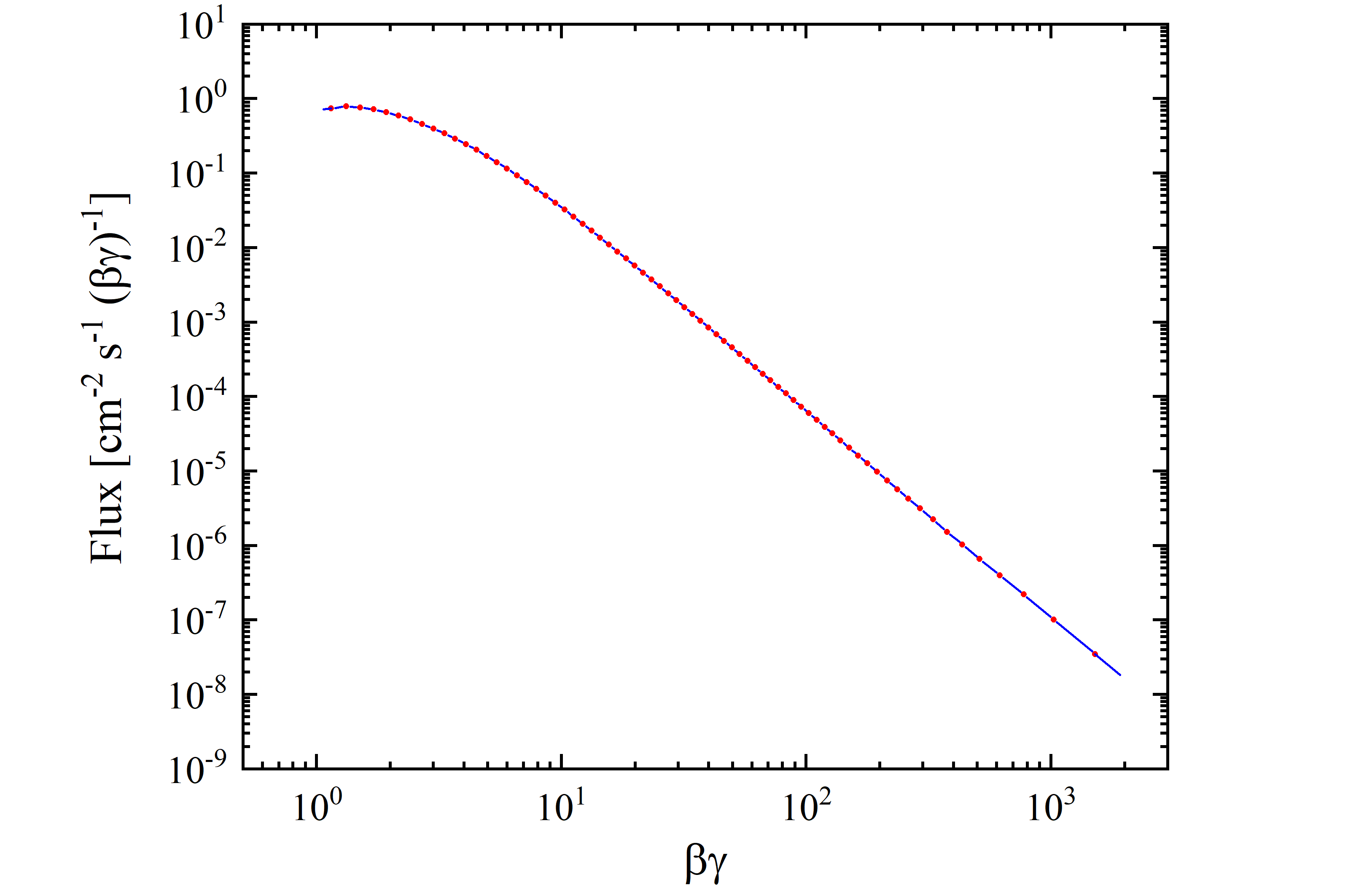 Figure 2. AMS02 proton flux data from [M. Aguilar et al. (2015)] as a function of βγ [see Eq. (1)]. Data points (red) are extracted from table 1. The interpolation line (blu) is shown from the lower limit of the first βγ bin (1.07) to the upper limit of the last one (1918.4).
The overall cosmic proton flux per unit area is 2.32 protons/[cm2 · s] from 433 MeV (βγ=1.07) up to 1.8 TeV (βγ=1918.4). As discussed above, the AMS-02 proton flux data covers a wide kinetic energy range from 433 MeV up 1.8 TeV, i.e., up to an upper energy limit which is much larger than that available from SRIM regarding stopping powers in absorbers. For instance, for protons the stopping powers in silicon is available up to an incoming energy of 10 GeV (βγ=11.61) - see SRIM Tutorials -. The integrated cosmic proton fluxes in protons/[cm2 · s] using AMS-02 data are reported in Table 2 as a function of energy (βγ) range.
| Energy [GeV] | βγ | Flux [cm2 s-1] | Fraction of Total Flux |
| 0.43 - 0.69 | 1.07 – 1.41 | 0.26 | 0.11 |
| 0.43 - 2.42 | 1.07 – 3.43 | 1.34 | 0.58 |
| 0.43 - 10.00 | 1.07 – 11.61 | 2.16 | 0.93 |
| 0.43 - 1800.00 | 1.07 – 1918.42 | 2.32 | 1.00 |
Table 2. Integrated cosmic proton flux per unit area iin protons/[cm2 · s] using AMS-02 data shown in Figures 2 and 3.
By an inspection of Table 2, it is worth to remark that above 10 GeV, the AMS-02 cosmic proton flux per unit area is 0.16 protons/[cm2 · s] - about 6.9% of the total -, i.e., the dominant fraction of the flux is that corresponding to protons with energies lower than 10 GeV. However, in such an energy region (below 10 GeV), the proton flux depends on the time dependent solar activity, i.e., modulation effects cannot be neglected (e.g., see the following discussion, see also www.helmod.org and, for instance, [Boschini et al 2019] and references therein).
Modulation effects on protons observed by AMS-02
The cosmic proton fluxes were observed on board od the International Space Station by AMS-02 from Bartels rotation 2426 (May 15, 2011 - June 10, 2011) up to Bartels rotation 2506 (April 13, 2017 - May 9, 2017) [[M. Aguilar et al. (2018)]]. In Table 3, as an example, the corresponding proton fluxes are shown for Bartels rotation 2464 (March 6, 2014 - April 1, 2014) and for 2506 (April 13, 2017 - May 9, 2017).
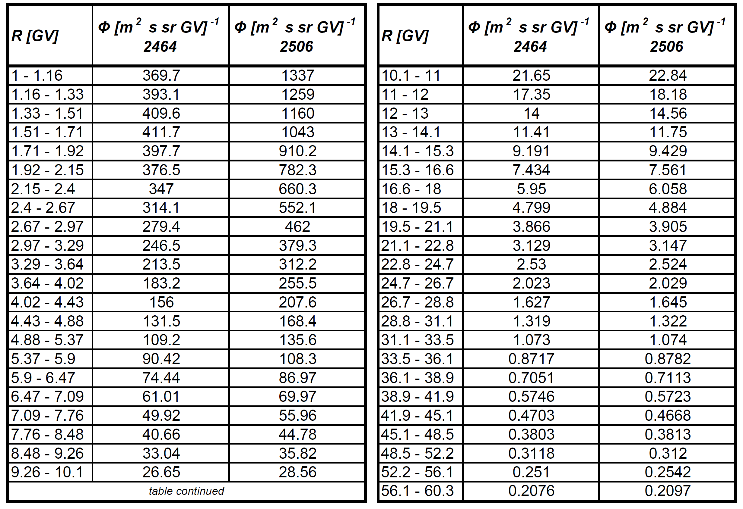
Table 3. Proton flux Φ in units of [m2 · sr · s · GV]−1as a function of rigidity at the top of AMS in units of [m2 · sr · s · GV]−1 for Bartels Rotation 2464 and 2506(from [M. Aguilar et al. (2018)]).
Using the data from Table 3, one finds that the total flux for Bartels rotation 2464 is 1.87 protons/[cm2 · s], for 2506 is 3.32 protons/[cm2 · s], i.e., the flux observed in the latter Bartels rotation was increased by about 77.5%. In addition, by an inspection of Table 3 one can note that for rigidities (e.g., see Eq. (1)) larger than about 16-20 GV the proton fluxes are similar in both Bartels rotation, i.e., the modulation effect is no longer affecting the protons transport within the heliosphere.
Properties of cosmic rays flux as a function of particle energy or electronic stopping power
The mass electronic stopping power for protons in silicon is shown as a function of kinetic energy (βγ) in figure 3 (4). It was calculated by means of the energy loss formula - Eq. (2.18) in Sect. 2.1.1 of [Leroy and Rancoita (2016)] - from 433 MeV (βγ=1.07) up to 1.8 TeV (βγ=1919.42) and was found in very good agreement with the values (red dashed curve) obained from SRIM (from which the mass electronic stopping power is available only up to 10 GeV). The stopping power exhibits a minimum for a kinetic energy of about 2.42 GeV) (i.e., for a βγ value of about 3.43).
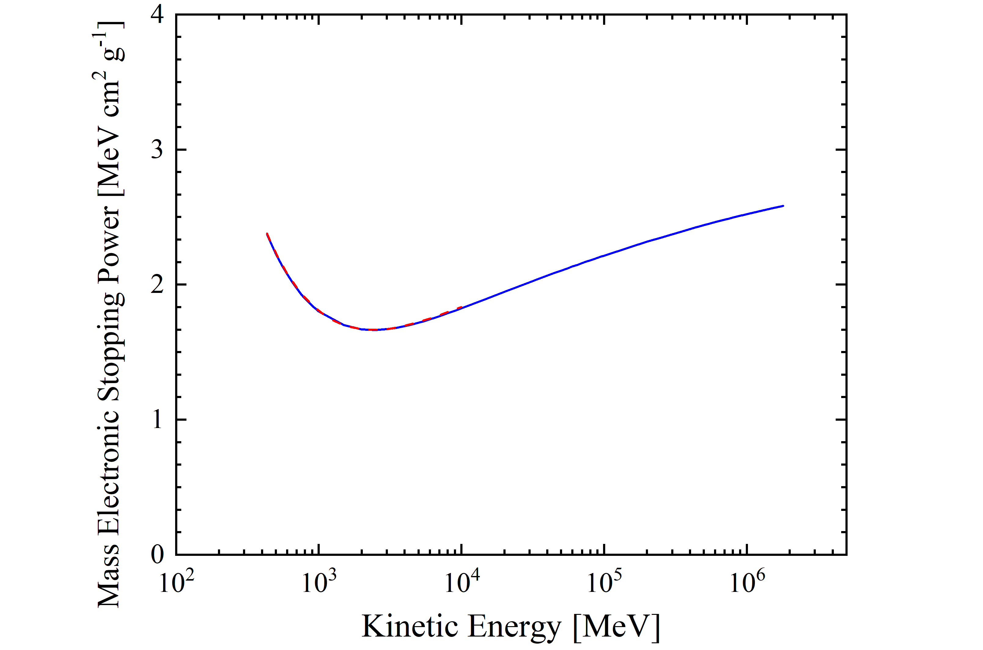
Figure 3. Mass electronic stopping power for protons in silicon as a function of kinetic energy. The blue solid curve is calculated with the energy loss formula - Eq. (2.18) in Sect. 2.1.1 of [Leroy and Rancoita (2016)] -. The red dashed curve is obtained from SRIM.
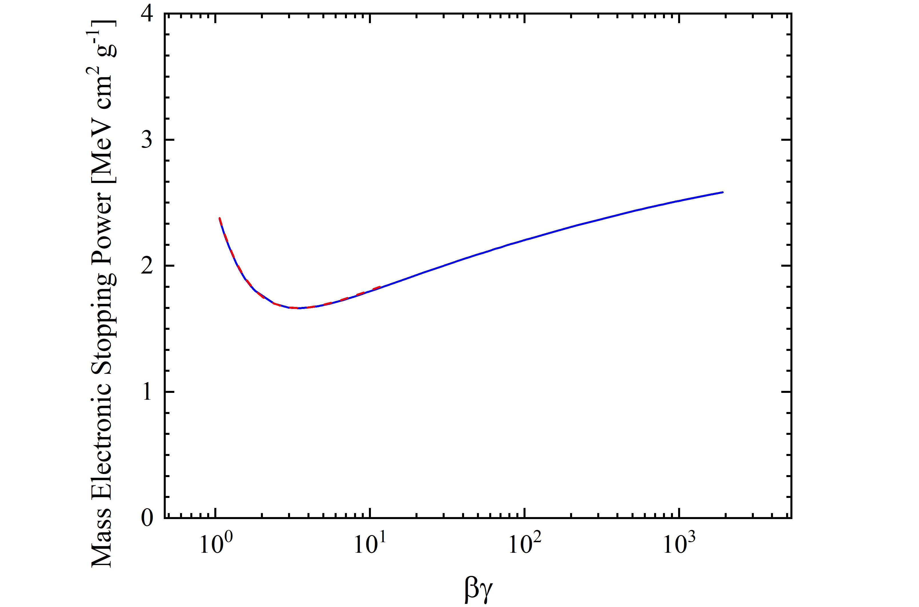
Figure 4. Mass electronic stopping power for protons in silicon as a function of βγ [see Eq. (1)]. The blue solid curve is calculated with the energy loss formula - Eq. (2.18) in Sect. 2.1.1 of [Leroy and Rancoita (2016)] -. The red dashed curve is obtained from SRIM.
From the observed cosmic proton fluxes of AMS-02 (previously discussed) as a function of the particle energy (or rigidity or βγ), one can derive those - Φ(ESP) - as a function of the mass electronic stopping power, i.e., in units of [MeV-1 · cm-4 · g · s-1], using the following expression which allows one to account correctly for the overall particle flux in each bin:![]()
where Φ(ESP) is the flux as a function of mass electronic stopping power, Φ(E) is the flux as a function of particle energy; ΔE and ΔESP are the extensions of the energy bin and of the corresponding mass electronic stopping power bin, respectively.
In Figures 5 and 6, the cosmic proton fluxes of AMS-02 are shown as a function of the mass electronic stopping power for four energy ranges indicated in Table 2. It has to be remarked that, because same values of mass electronic stopping power may be found at energy values lower and larger than the one corresponding to the ionization minimum (e.g., see Figure 3), the resulting shape of flux distribution depends on the energy range.
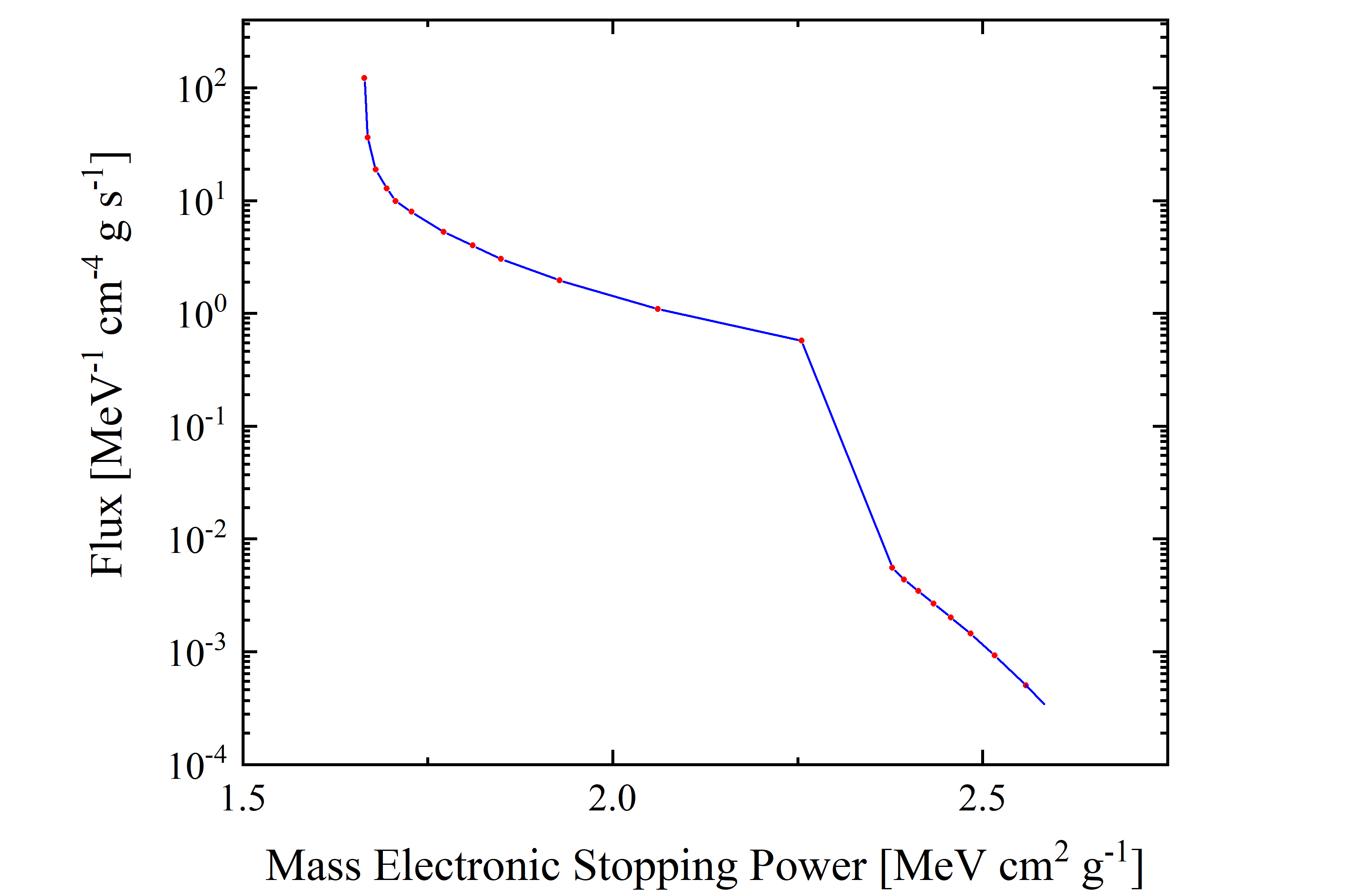
Figure 5. Cosmic Proton flux (observed by AMS-02, blue solid curve is the linear interpolation for the red data points) in units of [MeV-1 · cm-4 · g · s-1] as a function of mass electronic stopping power for protons in silicon in units of in units of [MeV · cm2 · g-1]; it corresponds to entire energy range with lower limit of 433 MeV and upper limit of 1.8 TeV.
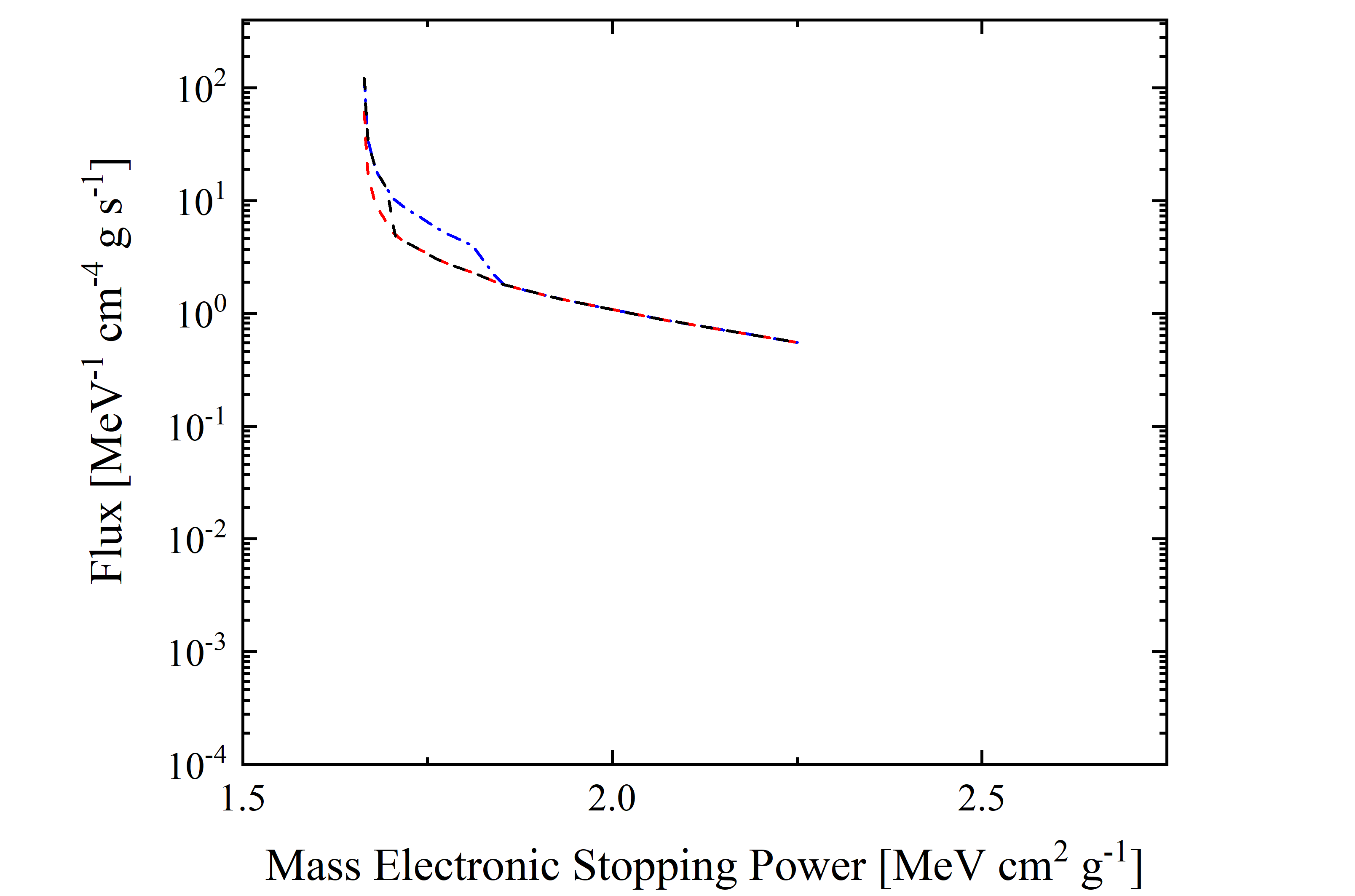
Figure 6. Cosmic Proton flux (observed by AMS-02) in units of [MeV-1 · cm-4 · g · s-1] as a function of mass electronic stopping power for protons in silicon in units of in units of [MeV · cm2 · g-1]; it corresponds to energy range with lower limit of 433 MeV and upper limit of 2.42 GeV (red dashed line), 4.44 GeV (black dashed line) and 10 GeV (blue dashed-dotted line).
The particle flux can be computed by integrating Φ(ESP) over the mass electronic stopping power range. The resulting values for the four curves shown in Figures 5 and 6 are listed in Table 4.
| integral particle using | Energy [GeV] | Flux [cm2 s-1] | Fraction of Total Flux |
| red dashed line (Figure 6) | 0.43 - 2.42 | 1.345 | 0.58 |
| black dashed line (Figure 6) | 0.43 - 4.44 | 1.808 | 0.78 |
| blue dashed-dotted line (Figure 6) | 0.43 - 10.00 | 2.156 | 0.93 |
| blue solid curve (Figure 5) | 0.43 - 1800.00 | 2.320 | 1.00 |
Table 4. Integrated cosmic proton flux per unit area in protons/[cm2 · s] using AMS-02 data shown in Figures 5 and 6.
By inspecting Tables 2 and 4, one can remarks that the in each energy range the particle fluxes - computed by integrating Φ(E) (see Figure 1) over the energy (see Table 2) and Φ(ESP) (see Figures 5 and 6) over the mass electronic stopping power (see Table 4) - are identical.
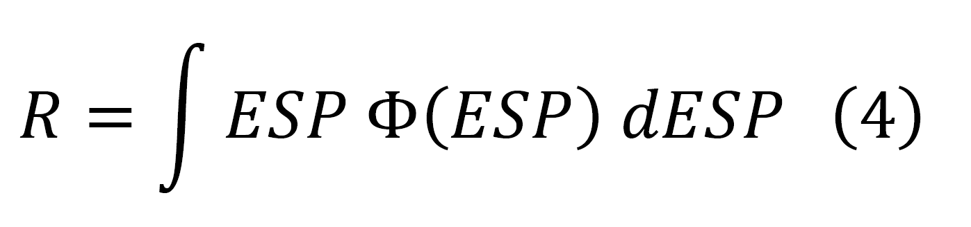
The equivalence of the two methodologies can also be inferred, for instance, in calculating the quantity R, i.e., the energy lost by the particles flux per g of traversed absorber. For each of the above discussed energy range, R can be computed using Φ(E) (see Table 5) as
![]()
where ESP is the mass electronic stopping power, or Φ(ESP) (see Table 6), i.e.,
| Energy [GeV] | R [MeV g-1 s-1] from Eq. (3) | Fraction of Total |
| 0.43 - 2.42 | 2.465 | 0.59 |
| 0.43 - 4.44 | 3.242 | 0.78 |
| 0.43 - 10.00 | 3.851 | 0.92 |
| 0.43 - 1800.00 | 4.168 | 1.00 |
Table 5. R values computed using Eq. (3).
| integral particle using | Energy [GeV] | R [MeV g-1 s-1] from Eq. (4) | Fraction of Total |
| red dashed line (Figure 6) | 0.43 - 2.42 | 2.465 | 0.59 |
| black dashed line (Figure 6) | 0.43 - 4.44 | 3.242 | 0.78 |
| blue dashed-dotted line (Figure 6) | 0.43 - 10.00 | 3.851 | 0.92 |
| blue solid curve (Figure 5) | 0.43 - 1800.00 | 4.168 | 1.00 |
Table 6. R values computed using Eq. (4).
By inspecting Tables 5 and 6, one can note that the R values do not depend on which methodology was used.
In summary, the two methodology (the former based on the original Φ(E) and the latter one with Φ(ESP) derived using Eq. (2)) result in providing the same value in each corresponding energy range. Thus, both of them can be equivalently employed.
Impact of employing the restricted energy-loss
In the above sections the treatment was focused on the energy lost by particles traversing a medium. However, in many physical processes - like those, for instance, regarding the so called single event effects (SEE) - the relevant energy is that deposited inside the absorber.
In fact, as discussed previously,since a device is usually not thick enough to fully absorb secondary δ-rays, the energy loss suffered by the incoming particle differs from the one deposited inside the detecting medium. As a consequence, the escaped δ-rays result in an effective detectable maximum transferred energy and, in turn, the deposited energy will reach a constant value, called the Fermi plateau at very high energy (for βγ > 744.7 (i.e., for protons with kinetic energies larger than 698 GeV). Thus, when the energy deposited into the device has to be dealt with -, one has to deal with the so called restricted energy loss in which the effective detectable maximum transferred energy is accounted for (e.g., see Sect. 2.1.1.4 in [Leroy and Rancoita (2016)]). Esbensen et al. (1978) have measured such an effect using silicon detector 900 μm thick and found a good agreement among experimental data and computed restricted energy-loss - from 690 MeV (βγ=1.41) - with the density-effect taken into account (see also [Rancoita (1984)] and here). The restricted energy loss from Esbensen et al. (1978) is shown in Figure 7 (8) as a function of proton kinetic energy (βγ) and found in good agreement with the curve obtained from the restricted energy loss formula (Eq. (2.29) in Sect. 2.1.1.4) from [Leroy and Rancoita (2016)] with W0 ≈ 0.5 MeV. One has to remark that restricted energy loss values for βγ > 100 (i.e., for protons with kinetic energies larger than 92.9 GeV) already approach that of the Fermi plateau within 0.5%.
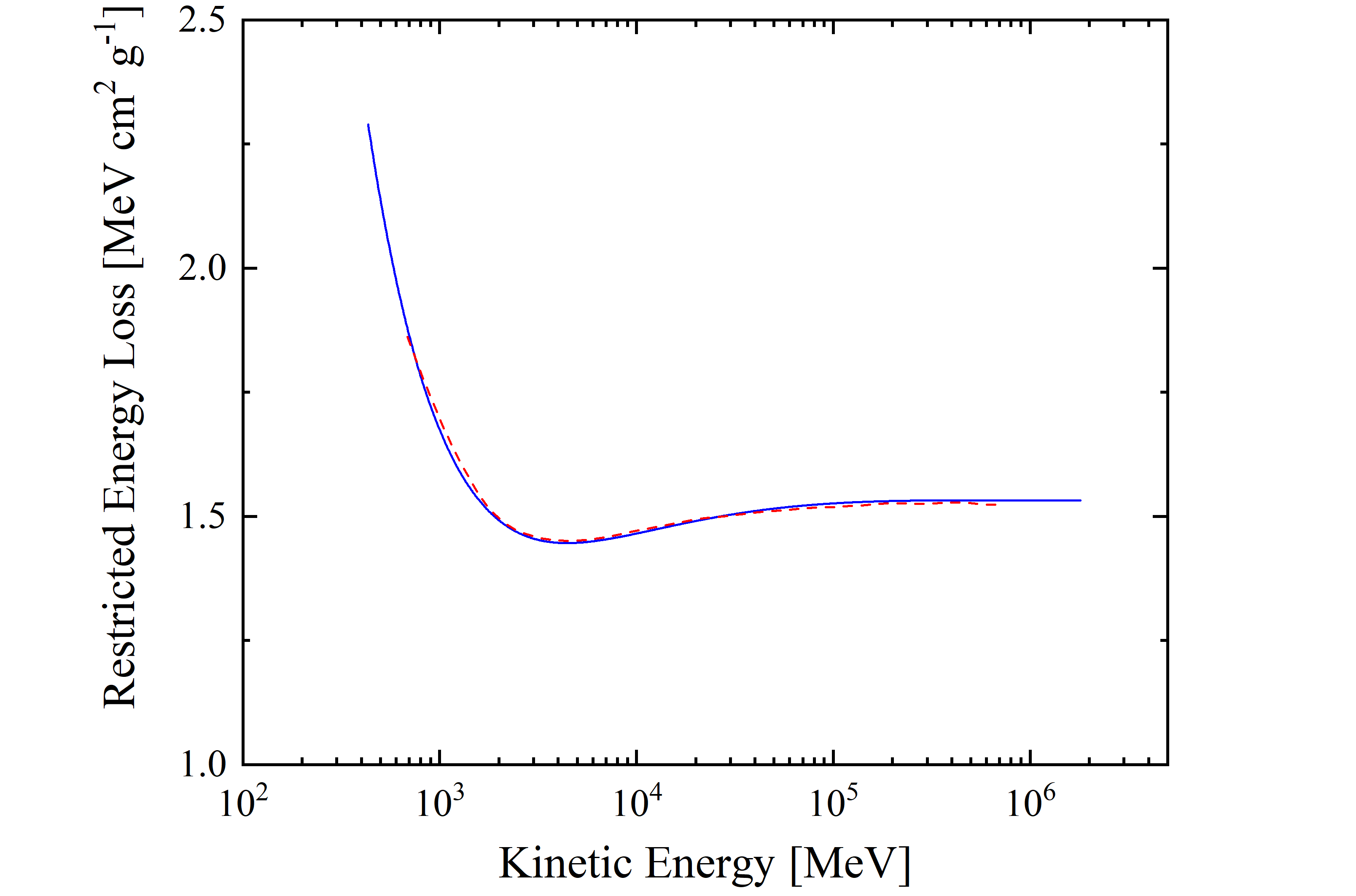 Figure 7. The restricted energy loss -from 433 MeV up to 18.TeV -for silicon detector 900 μm thick is shown as a function of proton kinetic energy; The blue solid curve is calculated with the restricted energy loss formula - Eq. (2.29) in Sect. 2.1.1.4 of [Leroy and Rancoita (2016)] with W0 ≈ 0.5 MeV -. The red dashed curve is from Esbensen et al. (1978); one has to remark that the restricted energy loss values for βγ > 100 (i.e., 92.9 GeV) already approach the Fermi plateau within 0.5%. The ionization minimum occurs at 4.44 GeV.
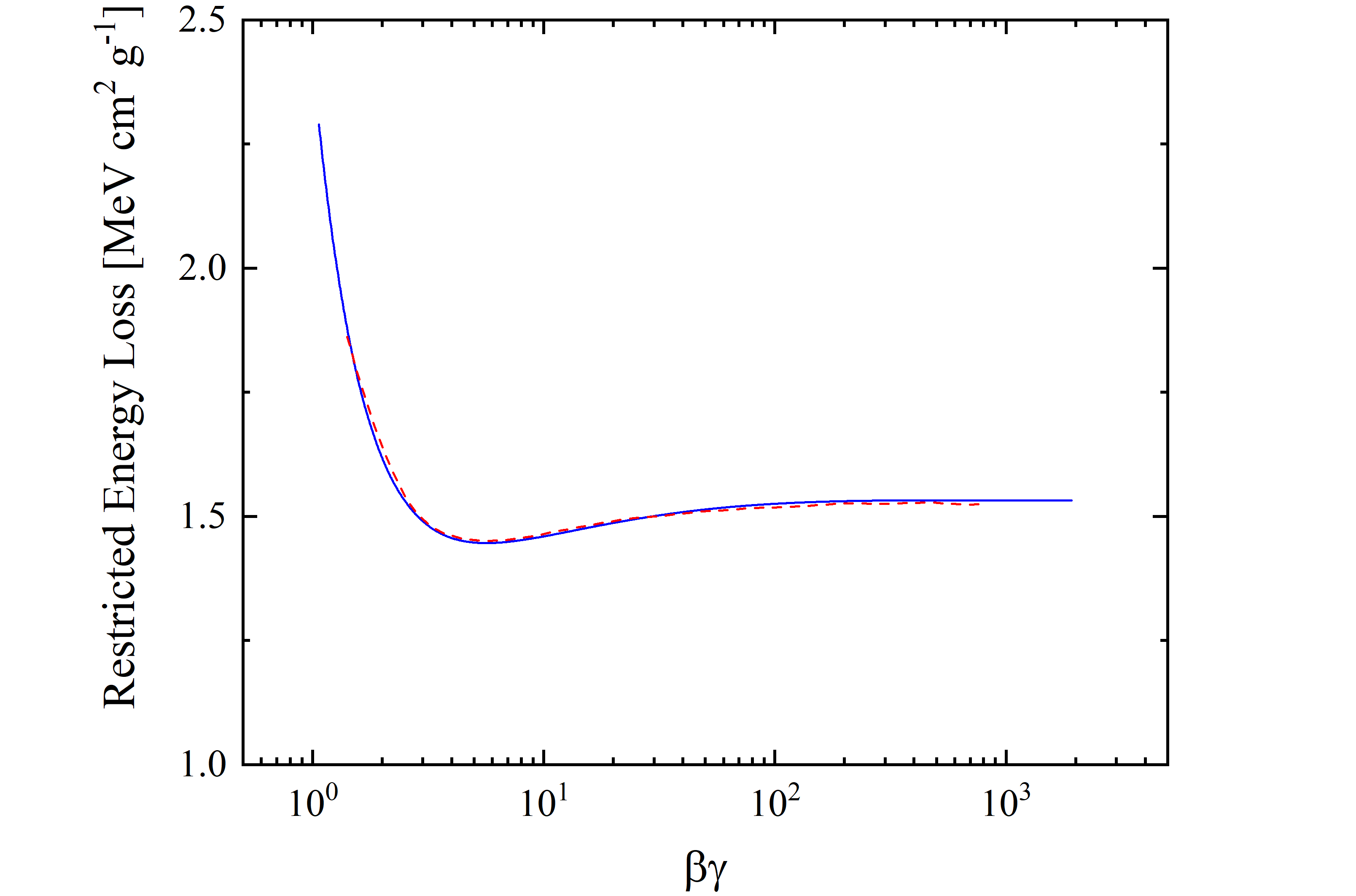 Figure 8. The restricted energy loss -from βγ=1.07 up to 1918.42 -for silicon detector 900 μm thick is shown as a function of βγ; The blue solid curve is calculated with the restricted energy loss formula - Eq. (2.29) in Sect. 2.1.1.4 of [Leroy and Rancoita (2016)] with W0 ≈ 0.5 MeV -. The red dashed curve is from Esbensen et al. (1978); one has to remark that the restricted energy loss values for βγ > 100 (i.e., 92.9 GeV) already approach the Fermi plateau within 0.5%. The ionization minimum occurs at βγ=5.65.
One has to remark that a) the restricted energy loss depends on the traversed path, therefore in the following we will consider particles impinging perpendicularly on the front side of the absorbing medium and b) that previous discussions - regarding mass electronic stopping power and the corresponding results reported in Figure 5 and 6, Tables 5 and 6 - apply also for perpendicularly impinging particles.
As already discussed, from the observed cosmic proton fluxes of AMS-02 (previously discussed) as a function of the particle energy (or rigidity or βγ), one can derive those - Φ(REL) - as a function of the restricted energy loss, i.e., in units of [MeV-1 · cm-4 · g · s-1], using the following expression which allows one to account correctly for the overall particle flux in each bin: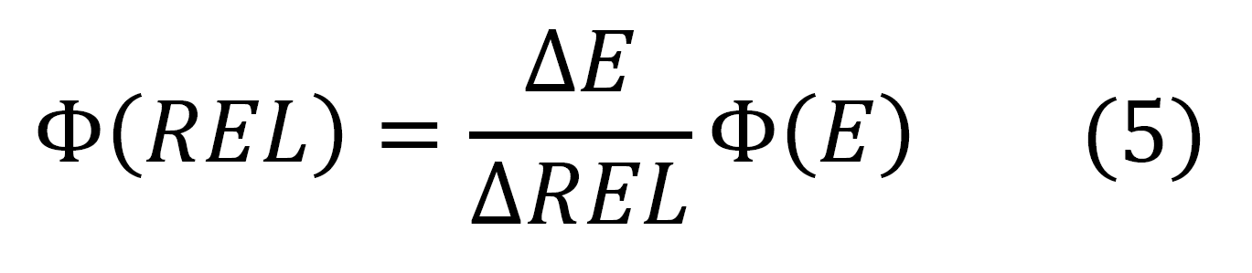
where Φ(REL) is the flux as a function of mass electronic stopping power, Φ(E) is the flux as a function of particle energy; ΔE and ΔREL are the extensions of the energy bin and of the corresponding restricted energy loss bin, respectively. In Figures 9 and 10, the cosmic proton fluxes of AMS-02 are shown as a function of the restricted energy loss for three energy ranges. It should be remarked that for βγ above 100 (i.e., for protons with kinetic energie larger than 92.9 GeV) ΔREL =0 and Eq. (5) is no longer valid, thus the corresponding particle flux cannot be accounted for.
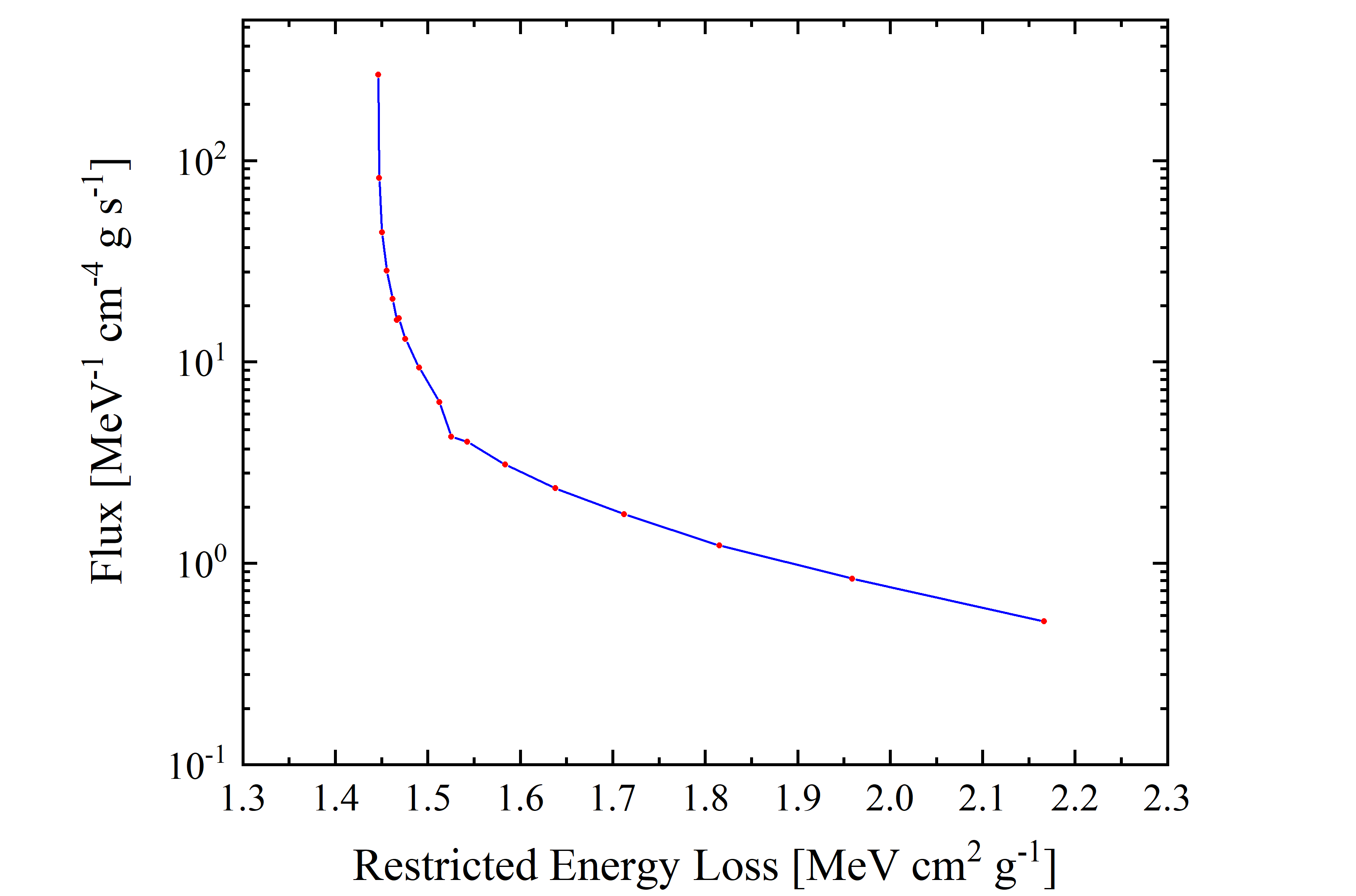 Figure 9. Cosmic Proton flux (observed by AMS-02, blue solid curve is the linear interpolation for the red data points) in units of [MeV-1 · cm-4 · g · s-1] as a function of restricted energy loss for protons in silicon in units of in units of [MeV · cm2 · g-1]; it corresponds to energy range with lower limit of 433 MeV and upper limit of 92.9 GeV. One has to remark that the restricted energy loss values for βγ > 100 is constant and gives no contribution since ΔREL = 0.
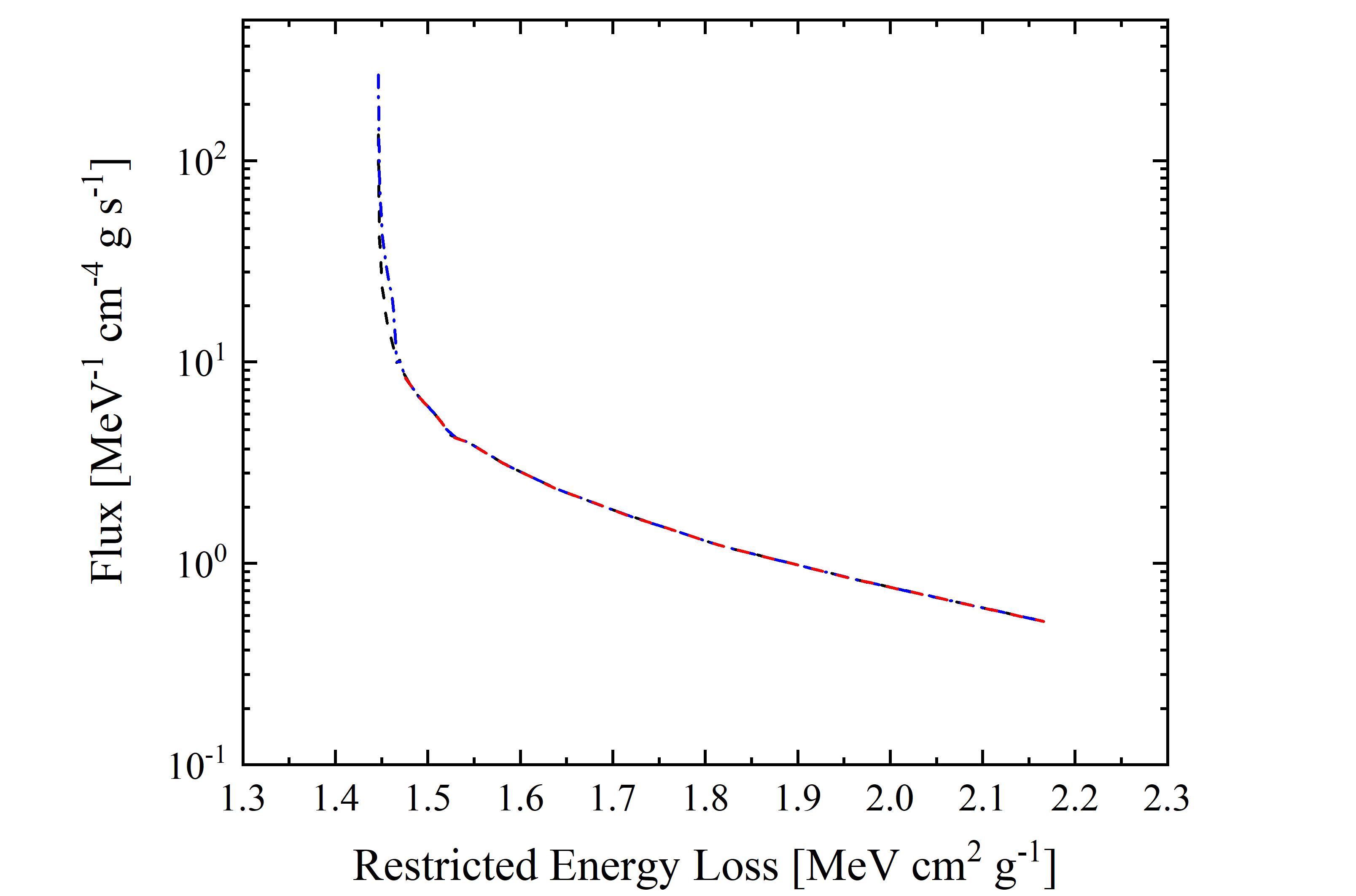 Figure 10. Cosmic Proton flux (observed by AMS-02) in units of [MeV-1 · cm-4 · g · s-1] as a function of mass electronic stopping power for protons in silicon in units of in units of [MeV · cm2 · g-1]; it corresponds to energy range with lower limit of 433 MeV and upper limit of 2.42 GeV (red dashed line), 4.44 GeV (black dashed line) and 10 GeV (blue dashed-dotted line). One has to remark that the restricted energy loss values for βγ > 100 is constant and gives no contribution since ΔREL = 0.
As treated previously, one compute the quantity R - i.e., the energy deposited by the particles flux per g of traversed absorber - for each energy range using Φ(E) (see Table 6) as
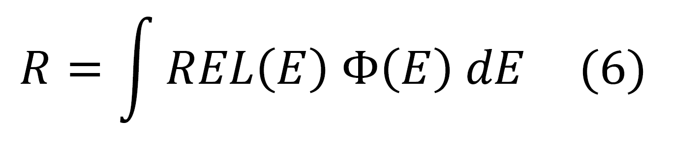
where REL is restricted energy loss, or Φ(REL) (see Table 7), i.e.,
![]()
| Energy [GeV] | βγ |
Flux [cm2 s-1] | R [MeV g-1 s-1] from Eq. (6) |
| 0.43 - 2.42 | 1.07 – 3.42 | 1.345 | 2.281 |
| 0.43 - 4.44 | 1.07 – 5.64 | 1.808 | 2.955 |
| 0.43 - 10.00 | 1.07 – 11.61 | 2.156 | 3.460 |
| 0.43 - 1800 | 1.07 – 1918.42 | 2.320 | 3.704 |
Table 6. R values computed using Eq. (6).
| integral particle using | Energy [GeV] | βγ | Flux [cm2 s-1] | R [MeV g-1 s-1] from Eq. (7) |
| red dashed line (Figure 10) | 0.43 - 2.42 | 1.07 – 3.42 | 1.345 | 2.281 |
| black dashed line (Figure 10) | 0.43 - 4.44 | 1.07 – 5.64 | 1.808 | 2.955 |
| blue dashed-dotted line (Figure 10) | 0.43 - 10.00 | 1.07 – 11.61 | 2.156 | 3.460 |
| blue solid curve (Figure 9) | 0.43 - 92.89 | 1.07 – 100.00 | 2.317 | 3.698 |
Table 7. R values computed using Eq. (7).
By inspecting Tables 6 and 7, one can note that the R values are almost unaffected - e.g., compare the fourth rows from Tables 6 and 7 - by not accounting the particles with βγ > 100, i.e., the usage of both Eqs. (6) and (7) provides similar results also when the deposited energy is taken in to account (e.g., see previous discussion). One can remark that by neglecting the particle flux above 10 GeV - i.e., taking into account the particle flux at energies where the solar modulation affects the particle transport within the heliosphere - the R value decreases by about 6.6% (e.g., see third and fourth rows in Tables 6) . In addition, the fluxes obtained in Table 2 and 6 are identical.
By comparing (Table 8) the R values obtained in Table 5 with those from Table 6, one finds that R is increased by a factor from 1.08 up to 1.13 (depending on the energy range taken into account), when the electronic stopping power replaces the restricted energy loss.
| Energy [GeV] | βγ |
Flux [cm2 s-1] | R [MeV g-1 s-1] from Eq. (6) | R [MeV g-1 s-1] from Eq. (3) |
Ratio |
| 0.43 - 2.42 | 1.07 – 3.42 | 1.345 | 2.281 | 2.465 | 1.08 |
| 0.43 - 4.44 | 1.07 – 5.64 | 1.808 | 2.955 | 3.242 | 1.10 |
| 0.43 - 10.00 | 1.07 – 11.61 | 2.156 | 3.460 | 3.851 | 1.11 |
| 0.43 - 1800 | 1.07 – 1918.42 | 2.320 | 3.704 | 4.168 | 1.13 |
Table 8. R values computed using Eq. (3) and (6).
Finally, one needs to note that the quantity R is cumulative and, thus, the impact might be different in case that a threshold quantity is investigated.
Bibliography
[M. Aguilar et al. (2015)] M. Aguilar et al., Phys. Rev. Lett. 114, 171103 (2015).
[M. Aguilar et al. (2018)] M. Aguilar et al., Phys. Rev. Lett. 121, 051101 (2018) and Observation of Fine Time Structures in the Cosmic Proton and Helium Fluxes with the Alpha Magnetic Spectrometer on the International Space Station - SUPPLEMENTAL MATERIAL -.
[Esbensen et al. (1978) Esbensen, H. et al. (1978). Phys. Rev. B 18, 1039.
[M.J. Boschini et al (2019)] M.J. Boschini, S. Della Torre, M. Gervasi, G. La Vacca and P.G. Rancoita, The HelMod Model in the Works for Inner and Outer Heliosphere: from AMS to Voyager Probes Observations, Advances in Space Res 64 (2019), 2459-2476 - https://doi.org/10.1016/j.asr.2019.04.007 -; available also at the website: https://arxiv.org/abs/1903.07501.
[Leroy and Rancoita (2016)] C. Leroy and P.G. Rancoita (2016), Principles of Radiation Interaction in Matter and Detection - 4th Edition -, World Scientific. Singapore, https://www.worldscientific.com/worldscibooks/10.1142/9167#t=aboutBook; ISBN-978-981-4603-18-8 (printed); ISBN.978-981-4603-19-5 (ebook); it is also partially accessible via google books.
[Rancoita (1984)] Rancoita, P.G. (1984). Silicon detectors and elementary particle physics, J. Phys. G: Nucl.Phys. 10, 299–319, doi: 10.1088/0305-4616/10/3/007.