

The current page is the update and the extension of the previous page, in which the comparison was limited to protons, helium-, lithium-, beryllium-, boron-, carbon-, nitrogen- and oxygen-nuclei.
The solar activity passes through low and high periods of activity (e.g., see NOAA space weather prediction center) every about 11 years (these are termed solar or sunspot cycles). Some time after a solar maximum, sun magnetic configuration is reversed e.g., see Svalgaard and Kamide, Asymmetric solar polar field reversals (2013)), so that it becomes similar every two solar cycles (termed Hale cycles or sometimes referred to as solar magnetic cycles), i.e., about 22 years. The properties of the solar wind (SW), such as its intensity and embedded magnetic field, are directly linked to solar activity. Parker in Dynamics of the Interplanetary Gas and Magnetic Fields (1958) suggested that the solar magnetic field is frozen-in to flow of the SW non-relativistic plasma, thereby creating the interplanetary magnetic field (IMF). This solar wind, a plasma primarily composed of protons constituting the largest amount of positively charged particles (e.g., see Ogilvie and Coplan, Solar wind composition (1995)), plays a pivotal role in modulating the intensities of galactic cosmic rays. It streams continuously from the Sun's corona to the boundaries of the heliosphere, exhibiting significant variability over time and space. Galactic cosmic rays (GCRs), with energies ranging from hundreds or less of MeV up to TeVs, are mostly responsible for damages due to SEEs in satellite subsystems mostly through the electronic stopping power process. Initially, the GCR transport through the heliosphere was addressed by Parker in the passage of energetic charged particles through interplanetary space (1965). In fact, the Parker Transport Equation, or Parker Equation, describes (1) the GCR diffusion by magnetic irregularities, (2) adiabatic energy changes related to cosmic radiation expansions and compressions, (3) the convection effect resulting from the solar wind velocity, and (4) drift effects linked to drift velocity. Drift velocity, crucially determined by the antisymmetric part of the diffusion tensor, depends on charge and Sun magnetic polarity configuration.
HelMod - the solar modulation model used within the SR-NIEL framework - is a well-known Monte Carlo code developed to describe the transport of GCRs through the heliosphere from interstellar space down to Earth (e.g., [HelMod (2022)], Chapter 8 of [Leroy and Rancoita (2016)]).
In the current HelMod version 4 the modulation process, based on Parker’s Equation, is applied to the propagation of GCRs in the inner and outer heliosphere, i.e., including the heliosheath. In fact, HelMod demonstrated to be capable of reproducing the fluxes observed by the Voyager probes in the inner and outer regions of the heliosphere up to its border. The HelMod model reproduced protons, antiprotons, nuclei, and electrons cosmic rays spectra observed - during solar cycles 23–24 and before - by several detectors, for instance, PAMELA, BESS, HEAO-3, ACE, and AMS-02 (e.g., see [HelMod (2022)] and Selected published HelMod spectra). In particular, the unprecedented accuracy of AMS-02 observations allowed one a better tuning of how solar modulation mechanisms are implemented inside the model.
In addition, HelMod can be used to forecast the GCRs omnidirectional intensities that space missions may encounter after the lift-off (see discussion in [Boschini et al. (2022a)]).
Furthermore, the join GalProp-HelMod (2016) effort allowed one to determine local interstellar spectra (LIS) of protons, antiprotons, ions, and electrons, whose set is gradually extended. The already available LISs of cosmic rays species - from which the HelMod modulated spectra can be derived - are listed on the HelMod website. There, in fact, a user can require the HelMod spectra for specific past and future periods or refer to published datasets (e.g., those from AMS-02, Pamela, etc.), i.e.,
- or single GCRs species and the future or past expected time interval can be chosen;
- or, for each published experimental dataset (e.g., those from AMS-02, Pamela, etc.), HelMod modulated spectra can be obtained regarding the time of observation, the type of investigated GCR species (e.g., proton, helium-nuclei, etc.), and, finally, the set of published data
In the present webpage (e.g., see Comparison of solar modulation models with experimental data from AMS-02), a selection of observed spectra of GCRs species are reported (see also [Boschini et al. (2022b)]), together with the modulated spectra obtained from some currently used solar modulation models, in particular dealing with space radiation environment, i.e.,
- CREME version 96 [CREME (1996)] and version 2009 (e.g., see [CREME (2012)]) using the CREME FLUX module as available from the CREME website upon registration;
- ISO-15390 model (e.g., see [ANSI (2004)]) using the package for galactic cosmic ray models as available from the SPENVIS website upon registration. This model is also suggested by the European Cooperation for Space Standardization (ECSS) for GRC differential flux calculations (see Section 9.2.3 of ECSS, 2020);
- BON2020 model (e.g. see [O’Neill et al. (2015)] and [Slaba&Whitman (2019)]) running the code on the OLTARIS website upon registration. At the time of the preparation of this webpage, the model is available only up to December 2018;
- HelMod (2022) model using the web calculator available from the HelMod website.
Selected published HelMod spectra and heliosphere
It has to be remarked that modulated spectra cannot be likely approximated uniform through the heliosphere (e.g. see Section 9.2.3 of ECSS, 2020) and depend on time and position.
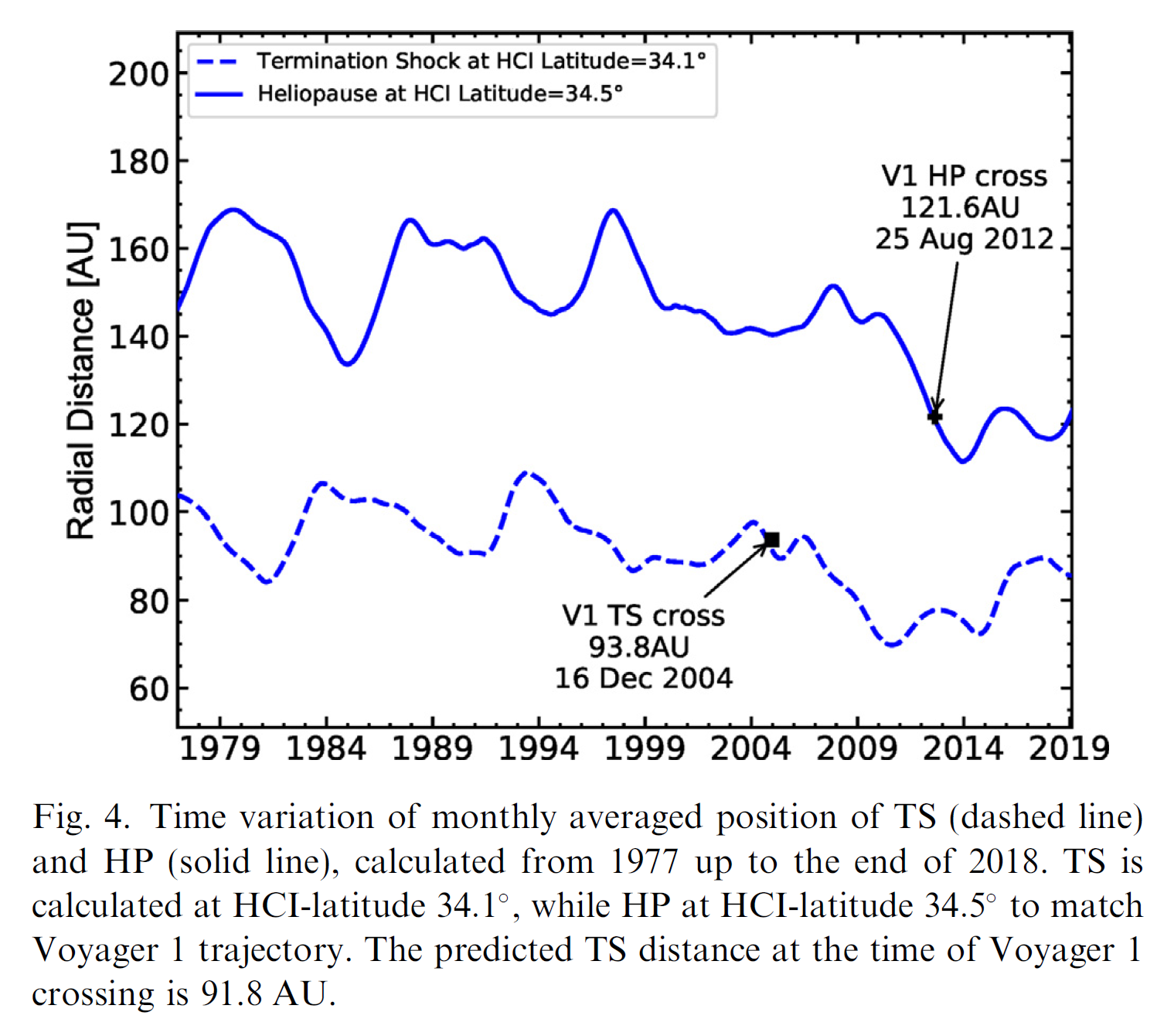
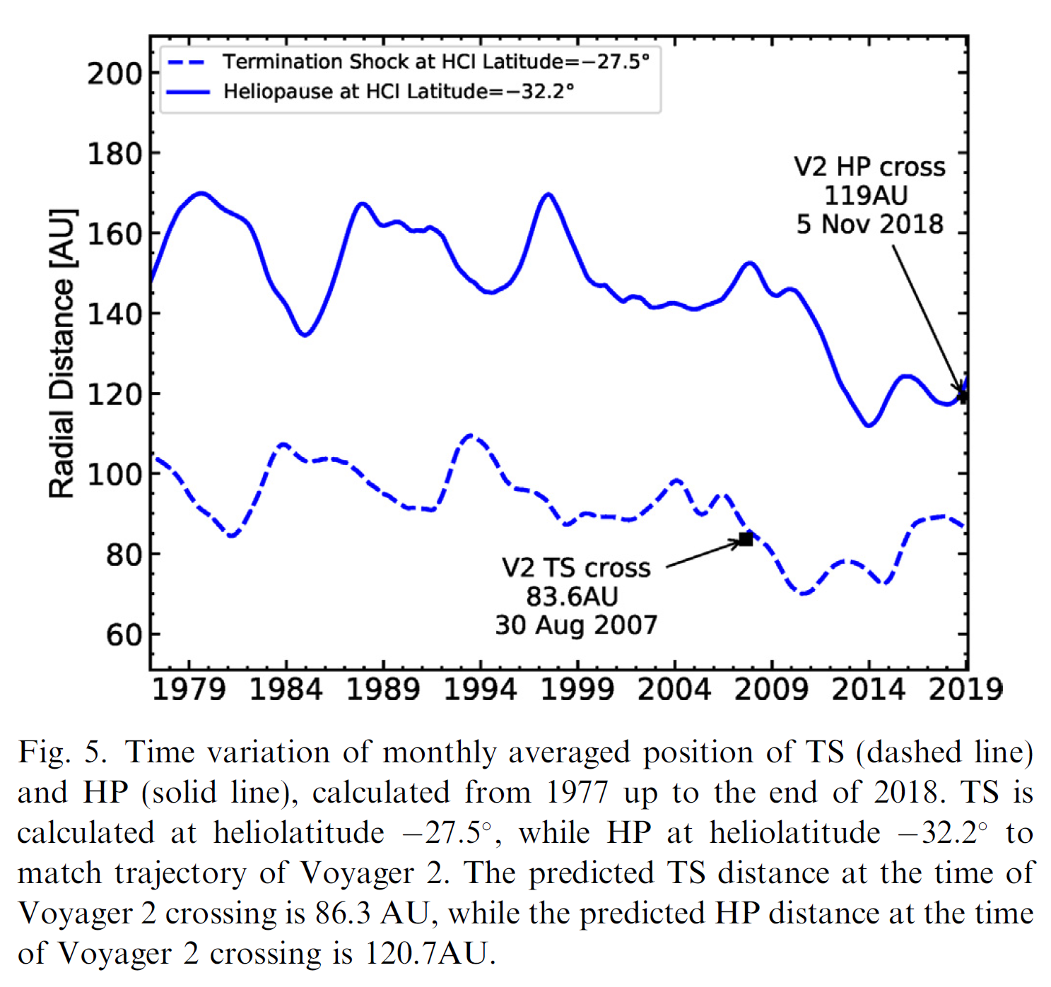
Figure 1. Reproduced from Figures 4 and 5 of [Boschini et al. (2019)].
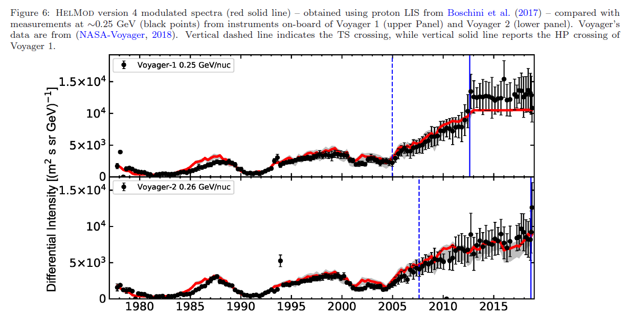
Figure 2. Reproduced from Figure 6 of [Boschini et al. (2019)].
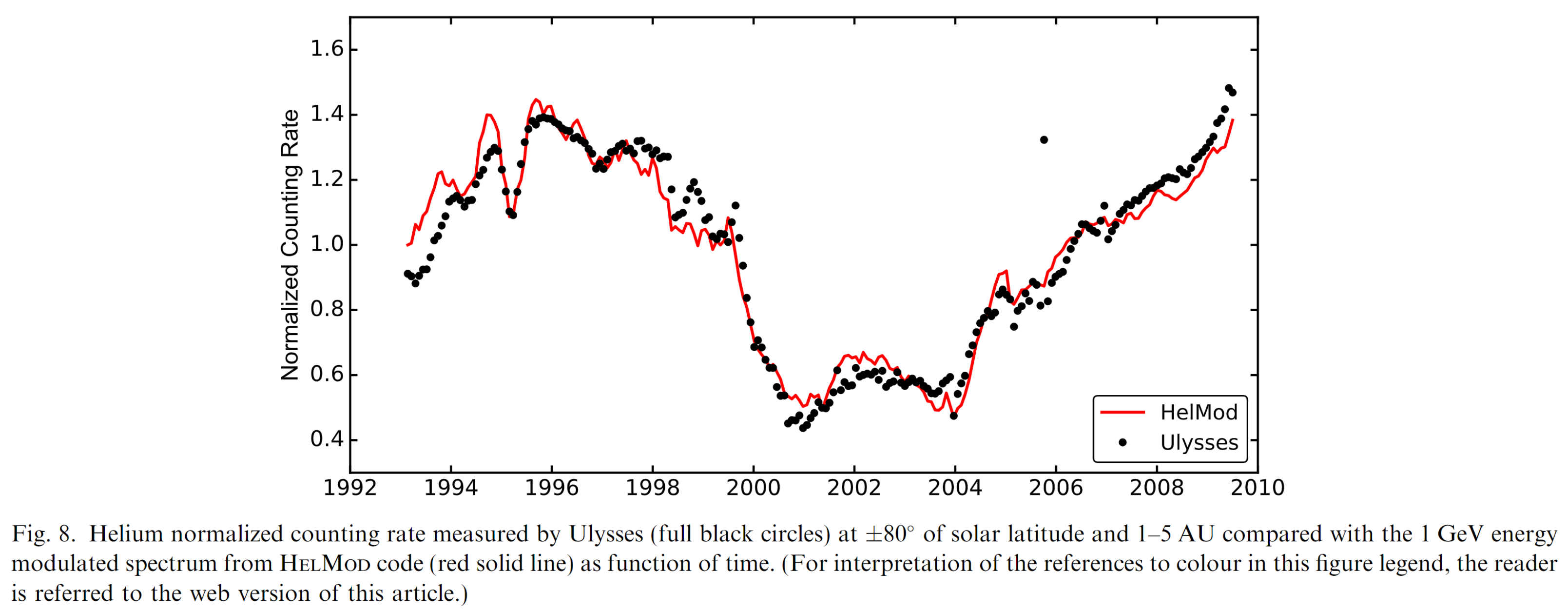
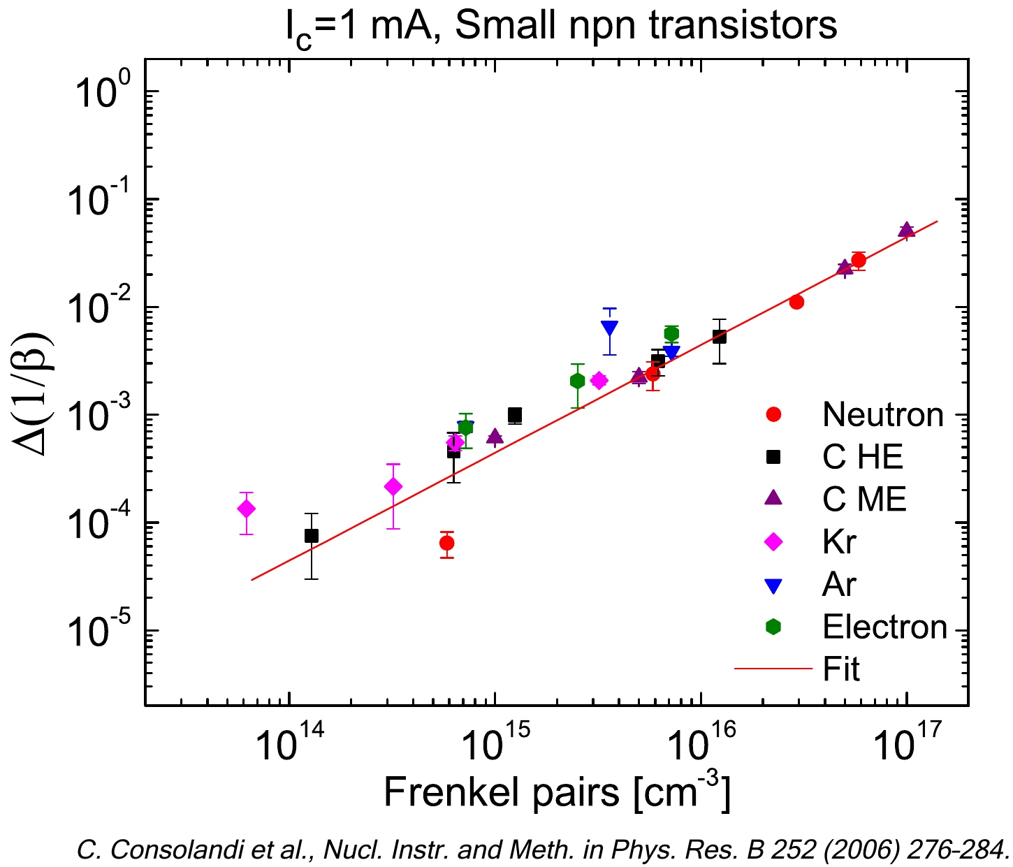
Figure 3. Reproduced from Figure 8 of [Boschini et al. (2018c)].
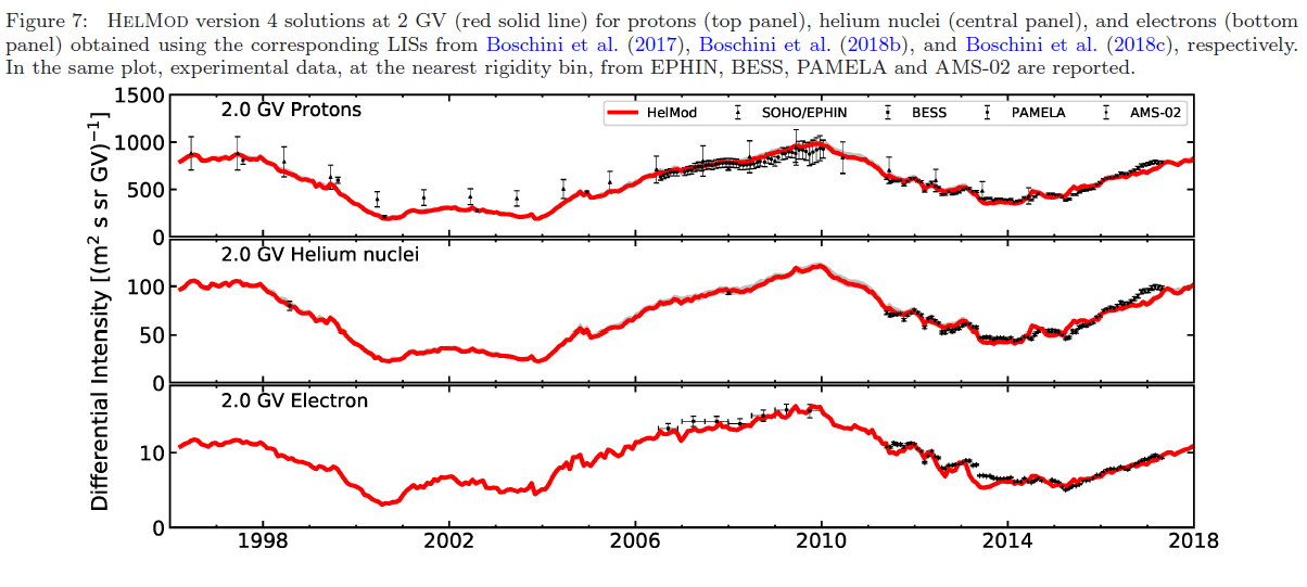
Figure 4. Reproduced from Figure 7 of [Boschini et al. (2019)].
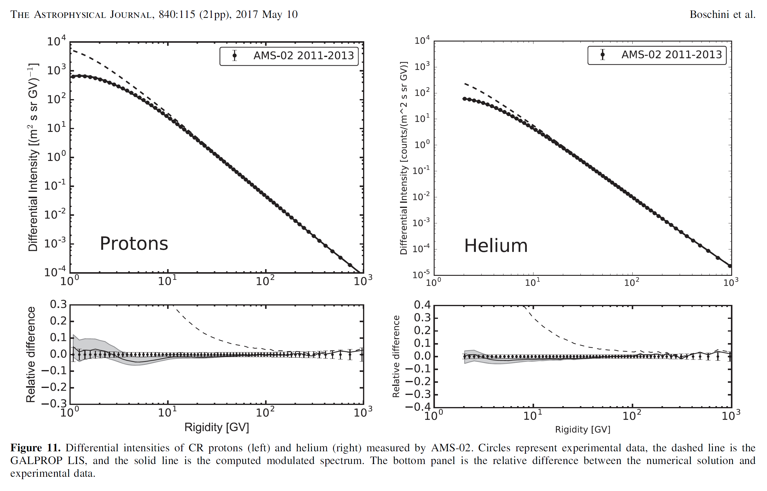
Figure 5. Reproduced from Figure 11 of [Boschini et al. (2017)]. AMS-02 proton data are from [Aguilar et al. (2015a)], AMS-02 helium data are from [Aguilar et al. (2015b)].

Figure 6. Reproduced from Figure 4 of [Boschini et al. (2018a)]. AMS-02 data (left panel) are from [Aguilar et al. (2014)], PAMELA data (right panel) are from [Adriani et al. (2011)].
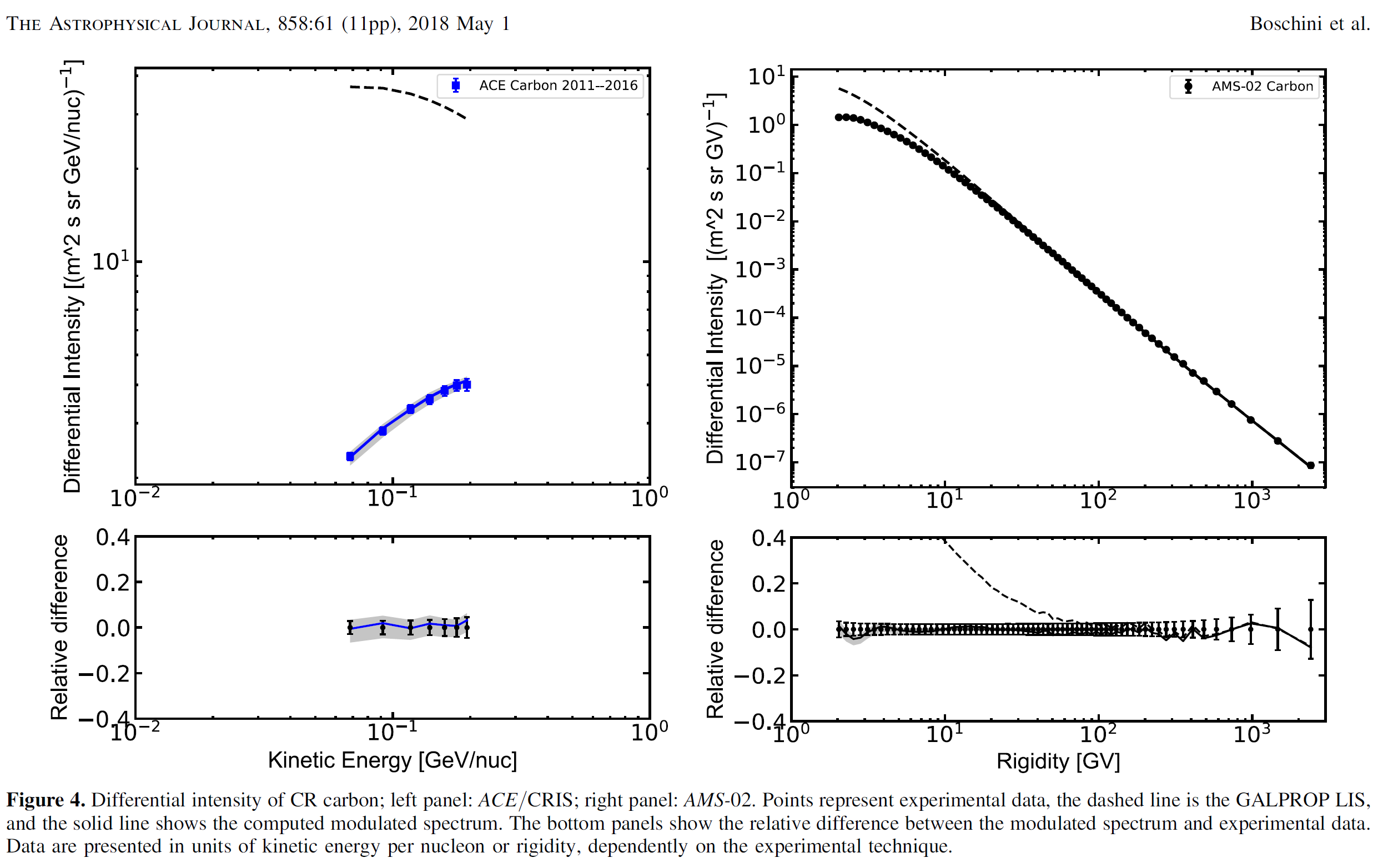
Figure 7. Reproduced from Figure 5 of [Boschini et al. (2018b)]. ACE data (left panel) are from [George et al. (2009)], AMS-02 data (right panel) are from [Aguilar et al. (2017)].
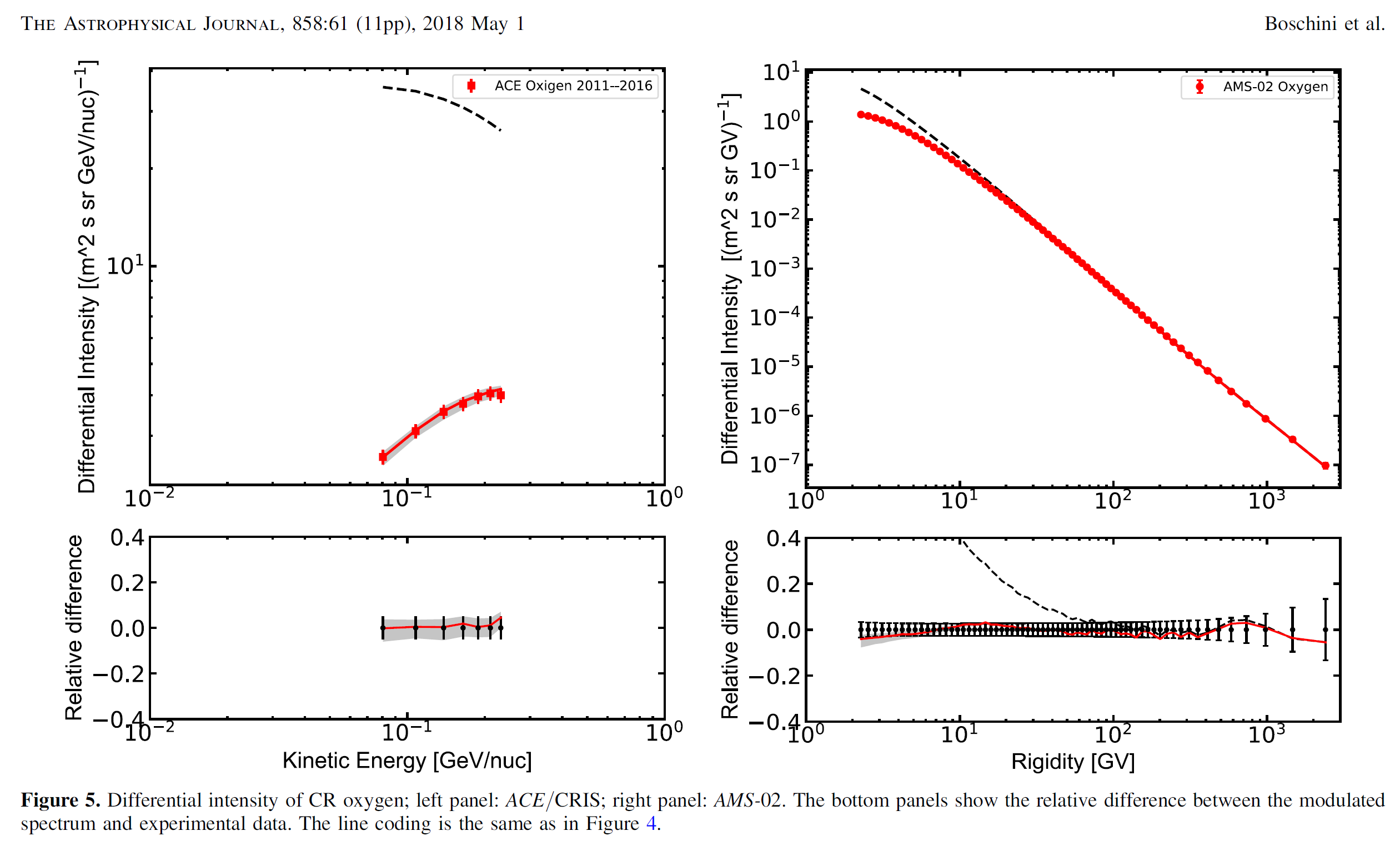
Figure 8. Reproduced from Figure 6 of [Boschini et al. (2018b)]. ACE data (left panel) are from [George et al. (2009)], AMS-02 data (right panel) are from [Aguilar et al. (2017)].
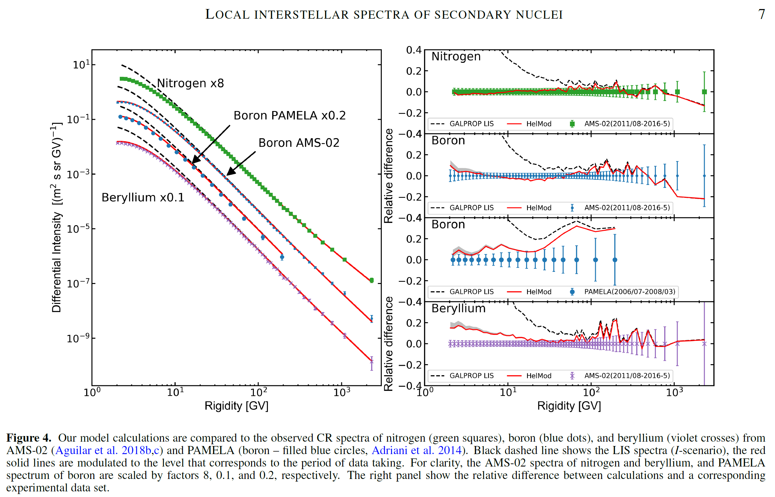
Figure 9. Reproduced from Figure 4 of [Boschini et al. (2020a)].
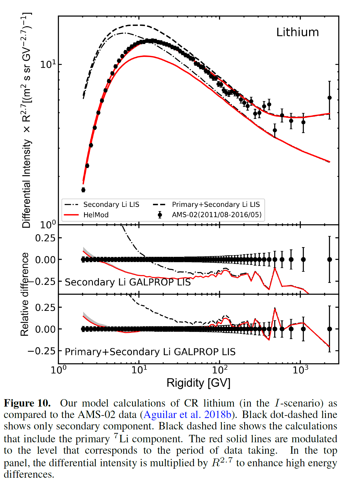
Figure 10. Reproduced from Figure 10 of [Boschini et al. (2020a)].
For further information on the results, please visit the HelMod results webpage.
Comparison of solar modulation models with experimental data from AMS-02
To benchmark several models (see the complete discussion in Boschini et al., 2022c), we considered the ion spectra measured by AMS–02 onboard the International Space Station (Aguilar et al., 2021a). AMS is a state-of-the-art particle detector providing the most accurate measurements of the GCR ion spectra exploiting its large acceptance and its excellent control of systematics. For the present webpage, we adopted the latest fluxes published by the Collaboration which reported the update of previously published GCR fluxes (Aguilar et al., 2021a) and the fluxes for Ne, Mg, Si (Aguilar et al., 2020) for the period up to May 26, 2018, and Fe (Aguilar et al., 2021b), F (Aguilar et al., 2021c), Na, Al (Aguilar et al., 2021d) ion fluxes for the period up to October 30, 2019. Due to the long exposure time and, thus, the high collected statistics, these measurements provide an improved measurement of the GCR spectra behavior at high rigidities.
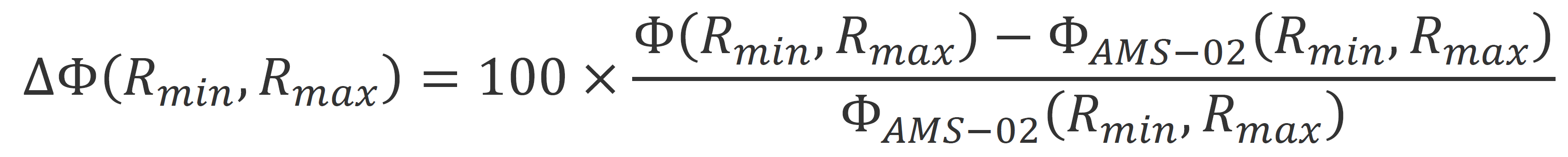
In the upper panels of Figures 9-23, the modulated spectra from CREME96, CREME2009, ISO-15390, and BON2020 are compared to both HelMod spectra and AMS02 data for protons, helium-, lithium-, beryllium-, boron-, carbon-, nitrogen-, oxygen-, neon-, magnesium-, silicon-, fluorine-, sodium-, aluminum-, iron-nuclei. As a function of rigidity R, relative differences of the solar model differential intensities, φ(R), with respect to that of AMS-02 data, φAMS-02(R), are calculated as
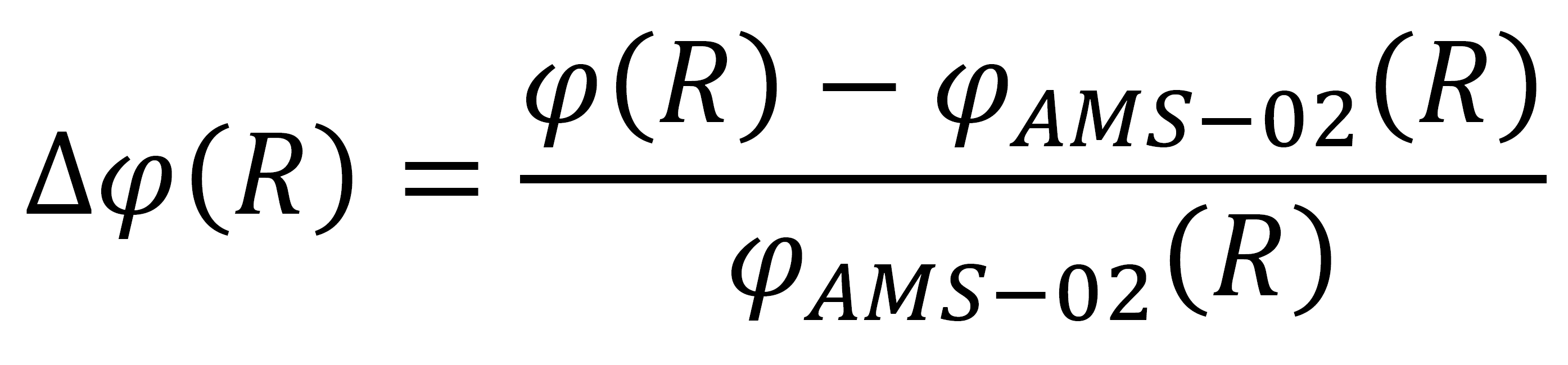 (1):
(1):
they are shown in the lower panels of the same figures.
{tab title="Fig. 11. Proton" class="blue"}
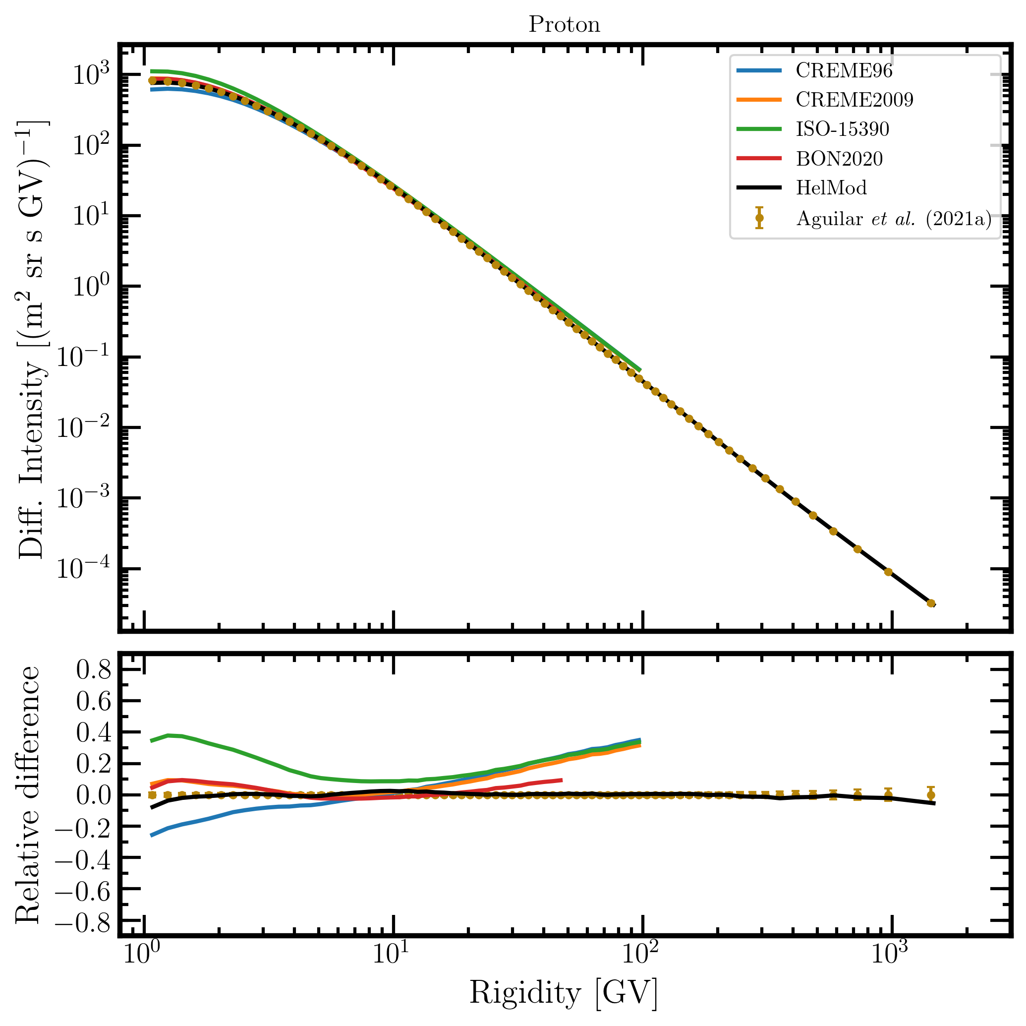
Figure 11. Upper panel: proton differential intensity in units of [m2 sr s GV]-1 measured by AMS-02 [Aguilar et al. (2021a)] (brown points) as a function of rigidity in GV from May 19, 2011, to November 26, 2018, and proton differential intensities - calculated at 1AU during the same period - for the presently investigated modulation models: CREME96 (blue curve), CREME2009 (orange curve), ISO-15390 (green curve), BON2020 (red curve) and HelMod (black curve). Lower panel: relative differences with respect to AMS-02 data calculated using Eq. (1). Adapted from Figure A5 and Figure 2 of Boschini et al. (2022c).
{tab title="Fig. 12. Helium" class="blue"} 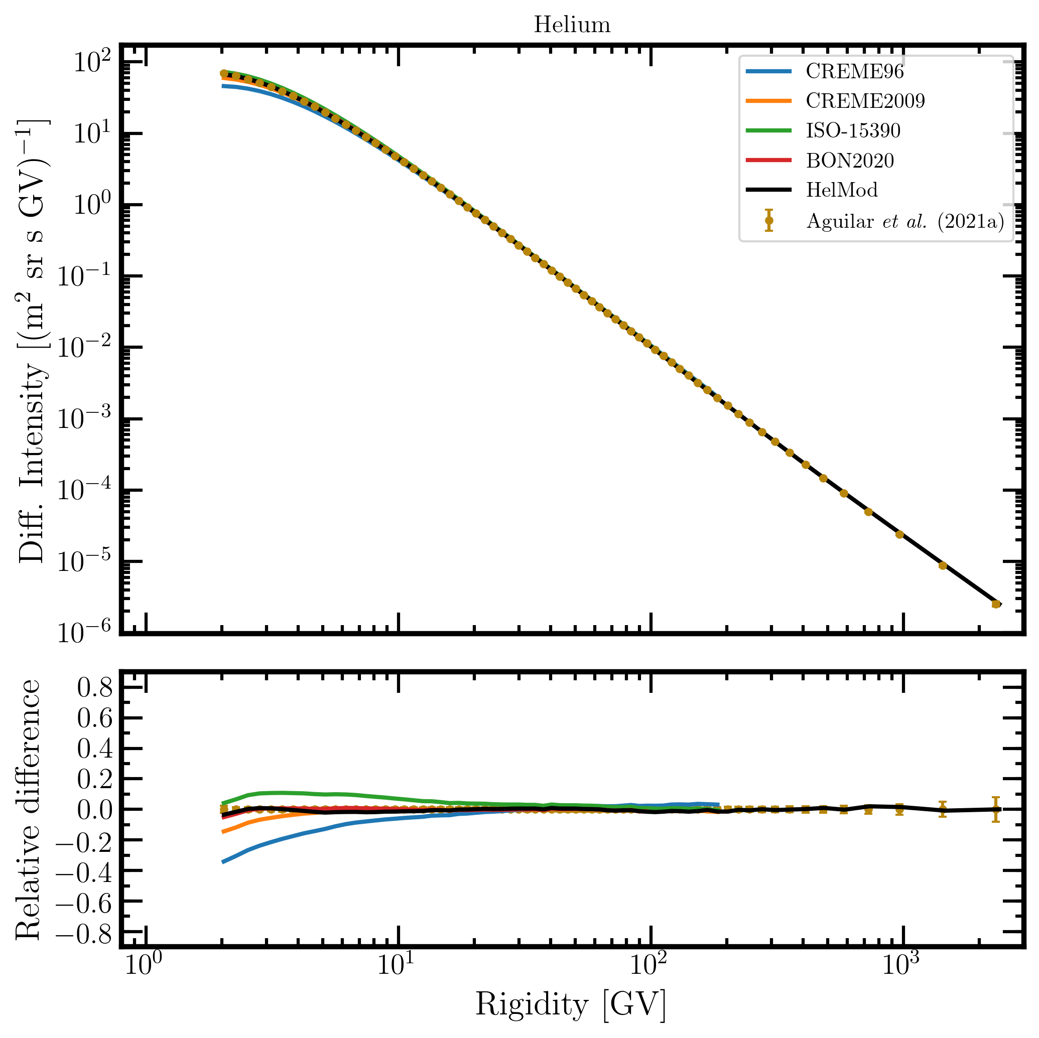
Figure 12. Upper panel: helium differential intensity in units of [m2 sr s GV]-1 measured by AMS-02 [Aguilar et al. (2021a)] (brown points) as a function of rigidity in GV from May 19, 2011, to November 26, 2018, and helium differential intensities - calculated at 1AU during the same period - for the presently investigated modulation models: CREME96 (blue curve), CREME2009 (orange curve), ISO-15390 (green curve), BON2020 (red curve) and HelMod (black curve). Lower panel: relative differences with respect to AMS-02 data calculated using Eq. (1). Adapted from Figure A6 and Figure 2 of Boschini et al. (2022c).
{tab title="Fig. 13. Lithium" class="blue"}
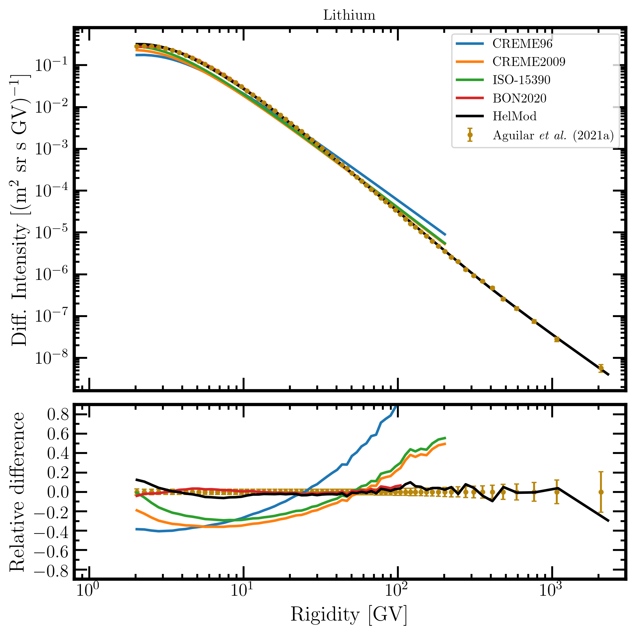
Figure 13. Upper panel: lithium differential intensity in units of [m2 sr s GV]-1 measured by AMS-02 [Aguilar et al. (2021a)] (brown points) as a function of rigidity in GV from May 19, 2011, to November 26, 2018, and lithium differential intensities - calculated at 1AU during the same period - for the presently investigated modulation models: CREME96 (blue curve), CREME2009 (orange curve), ISO-15390 (green curve), BON2020 (red curve) and HelMod (black curve). Lower panel: relative differences with respect to AMS-02 data calculated using Eq. (1). Adapted from Figure A7 and Figure 2 of Boschini et al. (2022c).
{tab title="Fig. 14. Beryllium" class="blue"}
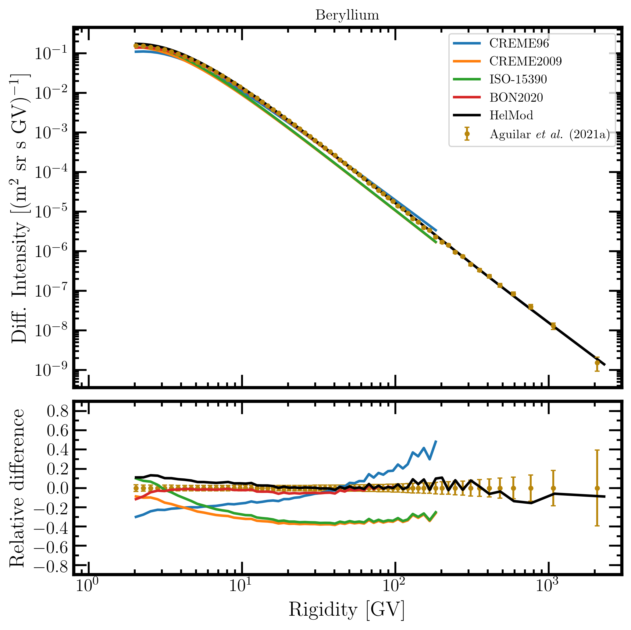
Figure 14. Upper panel: beryllium differential intensity in units of [m2 sr s GV]-1 measured by AMS-02 [Aguilar et al. (2021a)] (brown points) as a function of rigidity in GV from May 19, 2011, to November 26, 2018, and beryllium differential intensities - calculated at 1AU during the same period - for the presently investigated modulation models: CREME96 (blue curve), CREME2009 (orange curve), ISO-15390 (green curve), BON2020 (red curve) and HelMod (black curve). Lower panel: relative differences with respect to AMS-02 data calculated using Eq. (1). Adapted from Figure A8 and Figure 2 of Boschini et al. (2022c).
{tab title="Fig. 15. Boron" class="blue"}
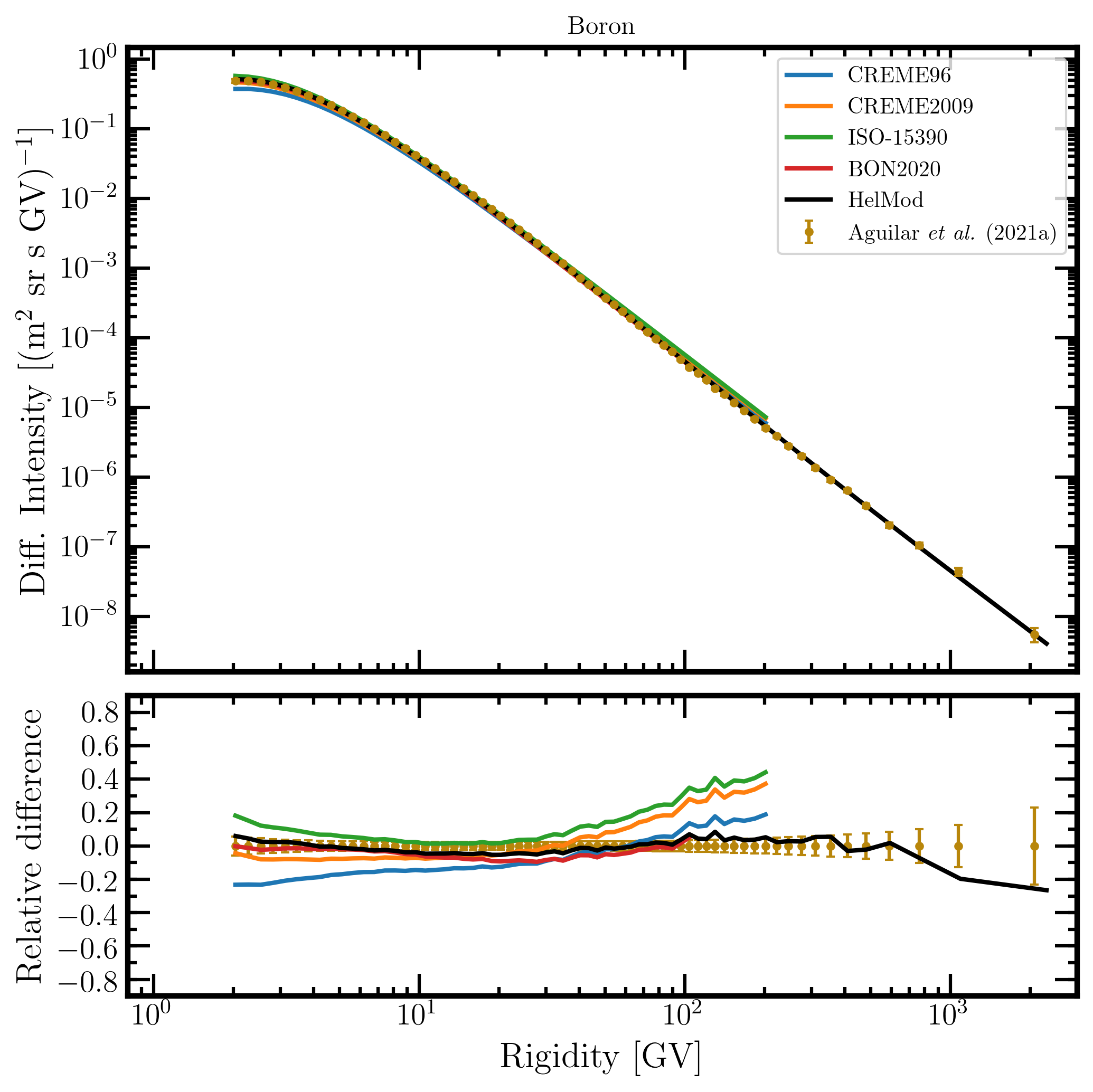
Figure 15. Upper panel: boron differential intensity in units of [m2 sr s GV]-1 measured by AMS-02 [Aguilar et al. (2021a)] (brown points) as a function of rigidity in GV from May 19, 2011, to November 26, 2018, and boron differential intensities - calculated at 1AU during the same period - for the presently investigated modulation models: CREME96 (blue curve), CREME2009 (orange curve), ISO-15390 (green curve), BON2020 (red curve) and HelMod (black curve). Lower panel: relative differences with respect to AMS-02 data calculated using Eq. (1). Adapted from Figure A9 and Figure 2 of Boschini et al. (2022c).
{tab title="Fig. 16. Carbon" class="blue"}
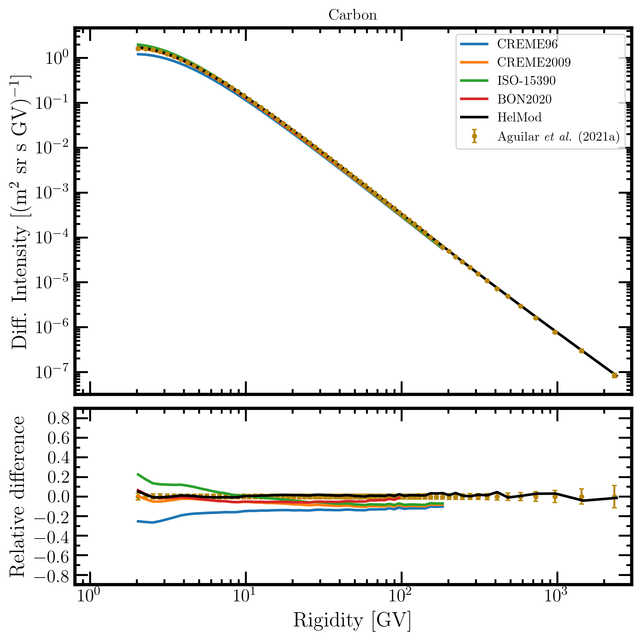
Figure 16. Upper panel: carbon differential intensity in units of [m2 sr s GV]-1 measured by AMS-02 [Aguilar et al. (2021a)] (brown points) as a function of rigidity in GV from May 19, 2011, to November 26, 2018, and carbon differential intensities - calculated at 1AU during the same period - for the presently investigated modulation models: CREME96 (blue curve), CREME2009 (orange curve), ISO-15390 (green curve), BON2020 (red curve) and HelMod (black curve). Lower panel: relative differences with respect to AMS-02 data calculated using Eq. (1). Adapted from Figure A10 and Figure 2 of Boschini et al. (2022c).
{tab title="Fig. 17. Nitrogen" class="blue"}
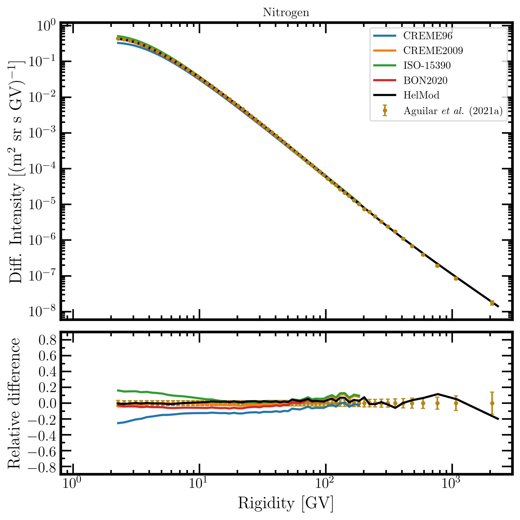
Figure 17. Upper panel: nitrogen differential intensity in units of [m2 sr s GV]-1 measured by AMS-02 [Aguilar et al. (2021a)] (brown points) as a function of rigidity in GV from May 19, 2011, to November 26, 2018, and nitrogen differential intensities - calculated at 1AU during the same period - for the presently investigated modulation models: CREME96 (blue curve), CREME2009 (orange curve), ISO-15390 (green curve), BON2020 (red curve) and HelMod (black curve). Lower panel: relative differences with respect to AMS-02 data calculated using Eq. (1). Adapted from Figure A11 and Figure 2 of Boschini et al. (2022c).
{tab title="Fig. 18. Oxygen" class="blue"}
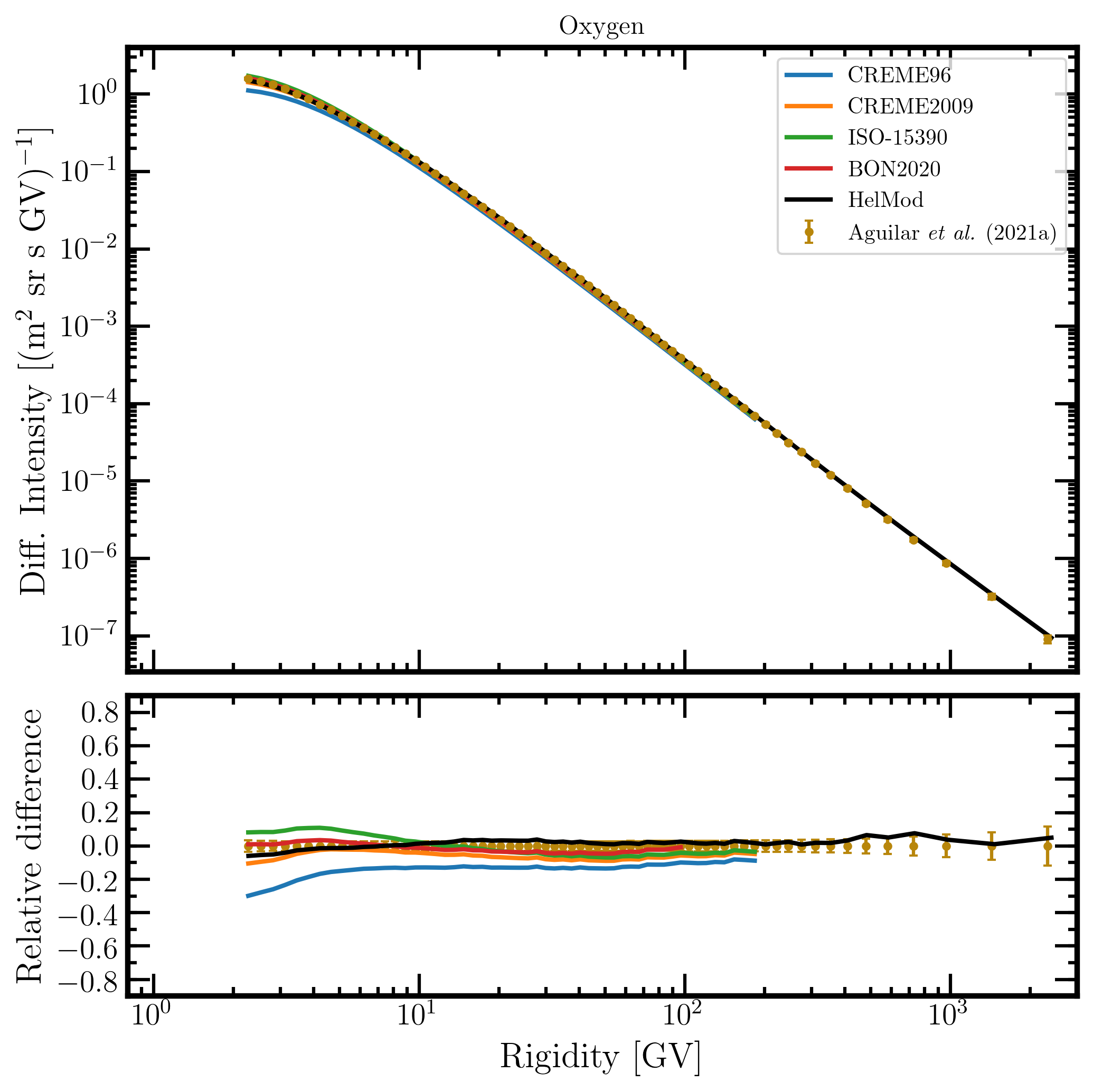
Figure 18. Upper panel: oxygen differential intensity in units of [m2 sr s GV]-1 measured by AMS-02 [Aguilar et al. (2021a)] (brown points) as a function of rigidity in GV from May 19, 2011, to November 26, 2018, and oxygen differential intensities - calculated at 1AU during the same period - for the presently investigated modulation models: CREME96 (blue curve), CREME2009 (orange curve), ISO-15390 (green curve), BON2020 (red curve) and HelMod (black curve). Lower panel: relative differences with respect to AMS-02 data calculated using Eq. (1). Adapted from Figure A12 and Figure 2 of Boschini et al. (2022c).
{tab title="Fig. 19. Fluorine" class="blue"}
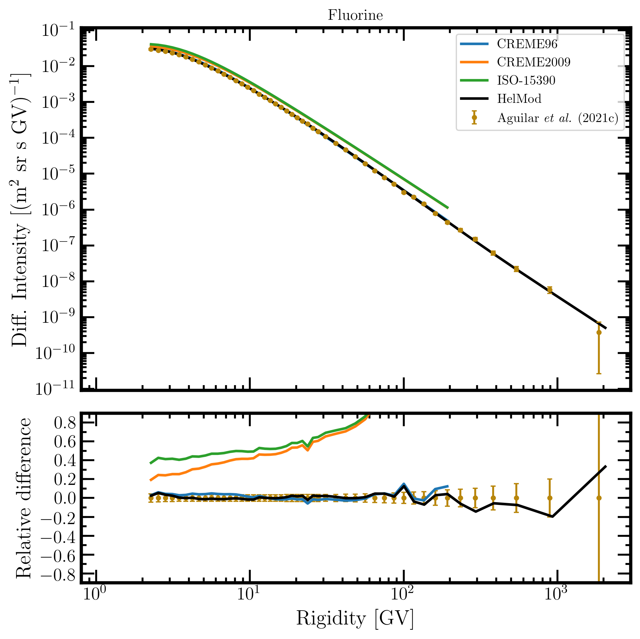
Figure 19. Upper panel: fluorine differential intensity in units of [m2 sr s GV]-1 measured by AMS-02 [Aguilar et al. (2021c)] (brown points) as a function of rigidity in GV from May 19, 2011, to October 30, 2019, and fluorine differential intensities - calculated at 1AU during the same period - for the presently investigated modulation models: CREME96 (blue curve), CREME2009 (orange curve), ISO-15390 (green curve), and HelMod (black curve). Lower panel: relative differences with respect to AMS-02 data calculated using Eq. (1). Adapted from Figure A13 and Figure 1 of Boschini et al. (2022c).
{tab title="Fig. 20. Neon" class="blue"}
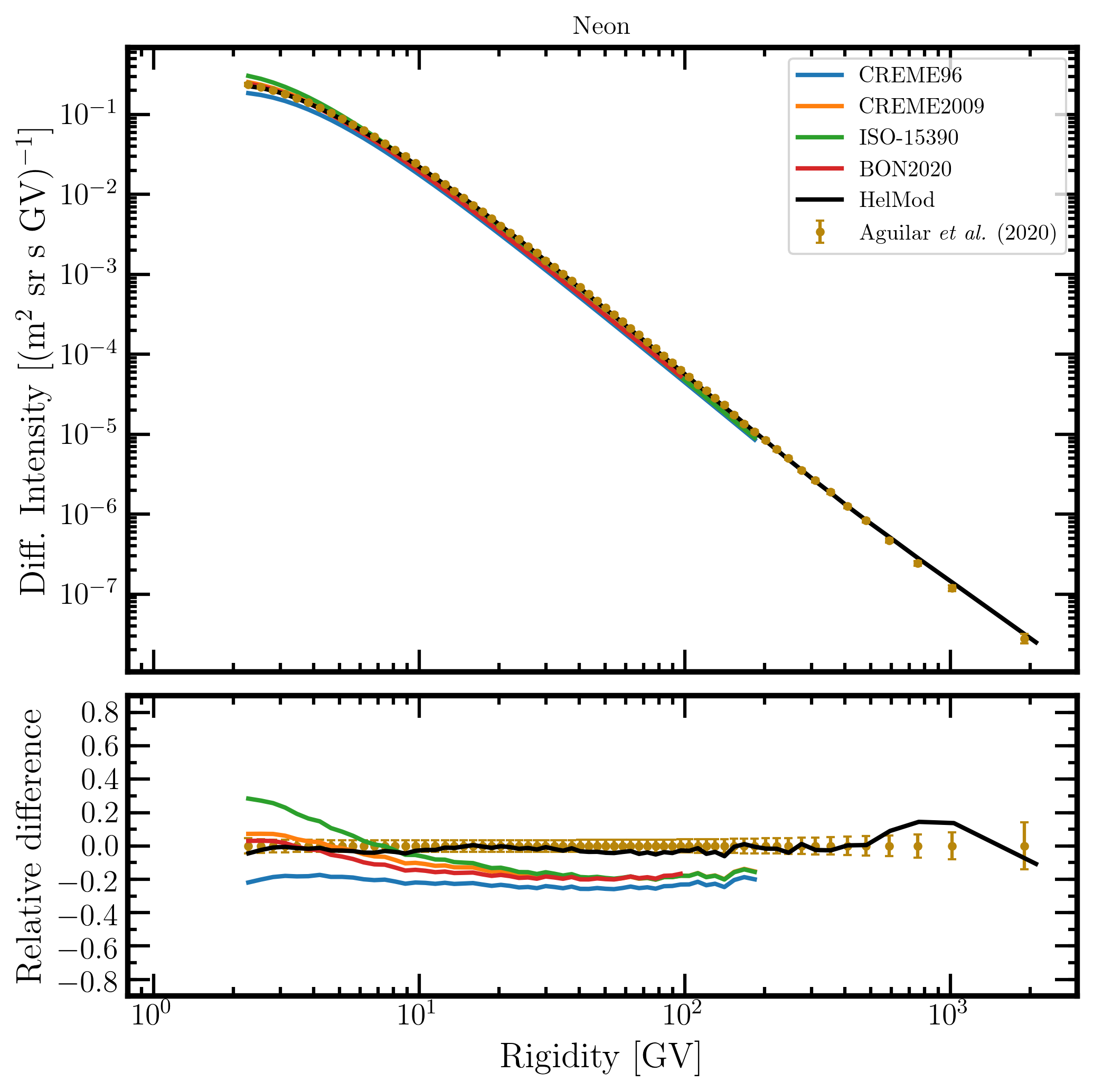
Figure 20. Upper panel: neon differential intensity in units of [m2 sr s GV]-1 measured by AMS-02 [Aguilar et al. (2020)] (brown points) as a function of rigidity in GV from May 19, 2011, to November 26, 2018, and neon differential intensities - calculated at 1AU during the same period - for the presently investigated modulation models: CREME96 (blue curve), CREME2009 (orange curve), ISO-15390 (green curve), BON2020 (red curve) and HelMod (black curve). Lower panel: relative differences with respect to AMS-02 data calculated using Eq. (1). Adapted from Figure A14 and Figure 2 of Boschini et al. (2022c).
{tab title="Fig. 21. Sodium" class="blue"}
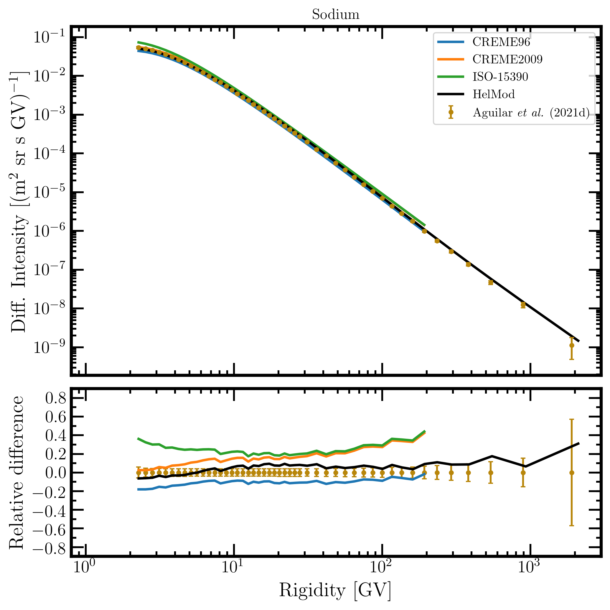
Figure 21. Upper panel: sodium differential intensity in units of [m2 sr s GV]-1 measured by AMS-02 [Aguilar et al. (2021d)] (brown points) as a function of rigidity in GV from May 19, 2011, to October 30, 2019, and sodium differential intensities - calculated at 1AU during the same period - for the presently investigated modulation models: CREME96 (blue curve), CREME2009 (orange curve), ISO-15390 (green curve), and HelMod (black curve). Lower panel: relative differences with respect to AMS-02 data calculated using Eq. (1). Adapted from Figure A15 and Figure 1 of Boschini et al. (2022c).
{tab title="Fig. 22. Magnesium" class="blue"}
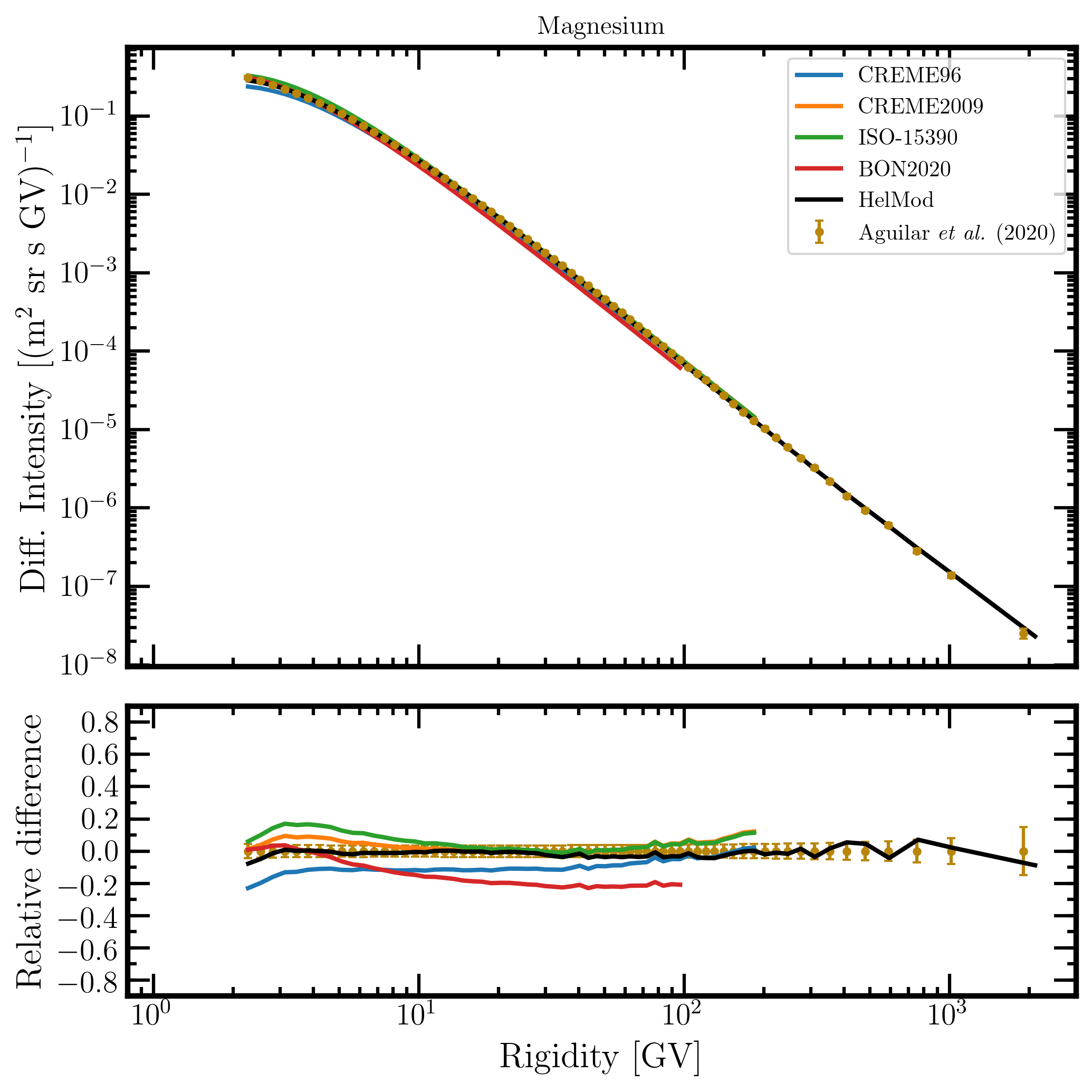
Figure 22. Upper panel: magnesium differential intensity in units of [m2 sr s GV]-1 measured by AMS-02 [Aguilar et al. (2020)] (brown points) as a function of rigidity in GV from May 19, 2011, to November 26, 2018, and magnesium differential intensities - calculated at 1AU during the same period - for the presently investigated modulation models: CREME96 (blue curve), CREME2009 (orange curve), ISO-15390 (green curve), BON2020 (red curve) and HelMod (black curve). Lower panel: relative differences with respect to AMS-02 data calculated using Eq. (1). Adapted from Figure A16 and Figure 2 of Boschini et al. (2022c).
{tab title="Fig. 23. Aluminum" class="blue"}
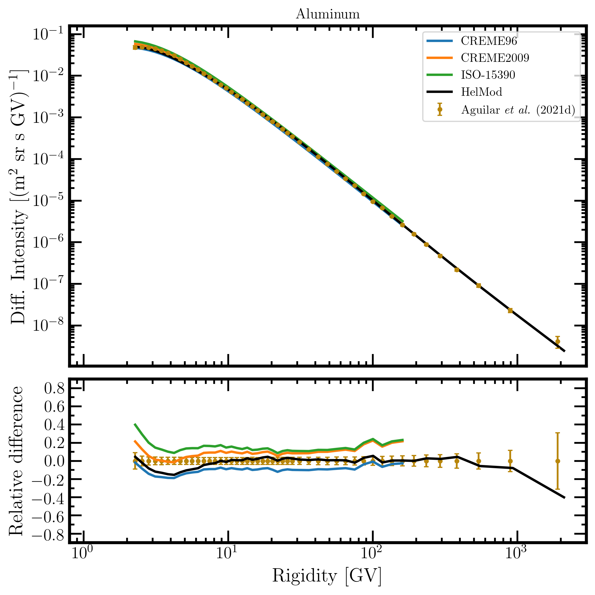
Figure 23. Upper panel: aluminum differential intensity in units of [m2 sr s GV]-1 measured by AMS-02 [Aguilar et al. (2021d)] (brown points) as a function of rigidity in GV from May 19, 2011, to October 30, 2019, and aluminum differential intensities - calculated at 1AU during the same period - for the presently investigated modulation models: CREME96 (blue curve), CREME2009 (orange curve), ISO-15390 (green curve), and HelMod (black curve). Lower panel: relative differences with respect to AMS-02 data calculated using Eq. (1). Adapted from Figure A17 and Figure 1 of Boschini et al. (2022c).
{tab title="Fig. 24. Silicon" class="blue"}
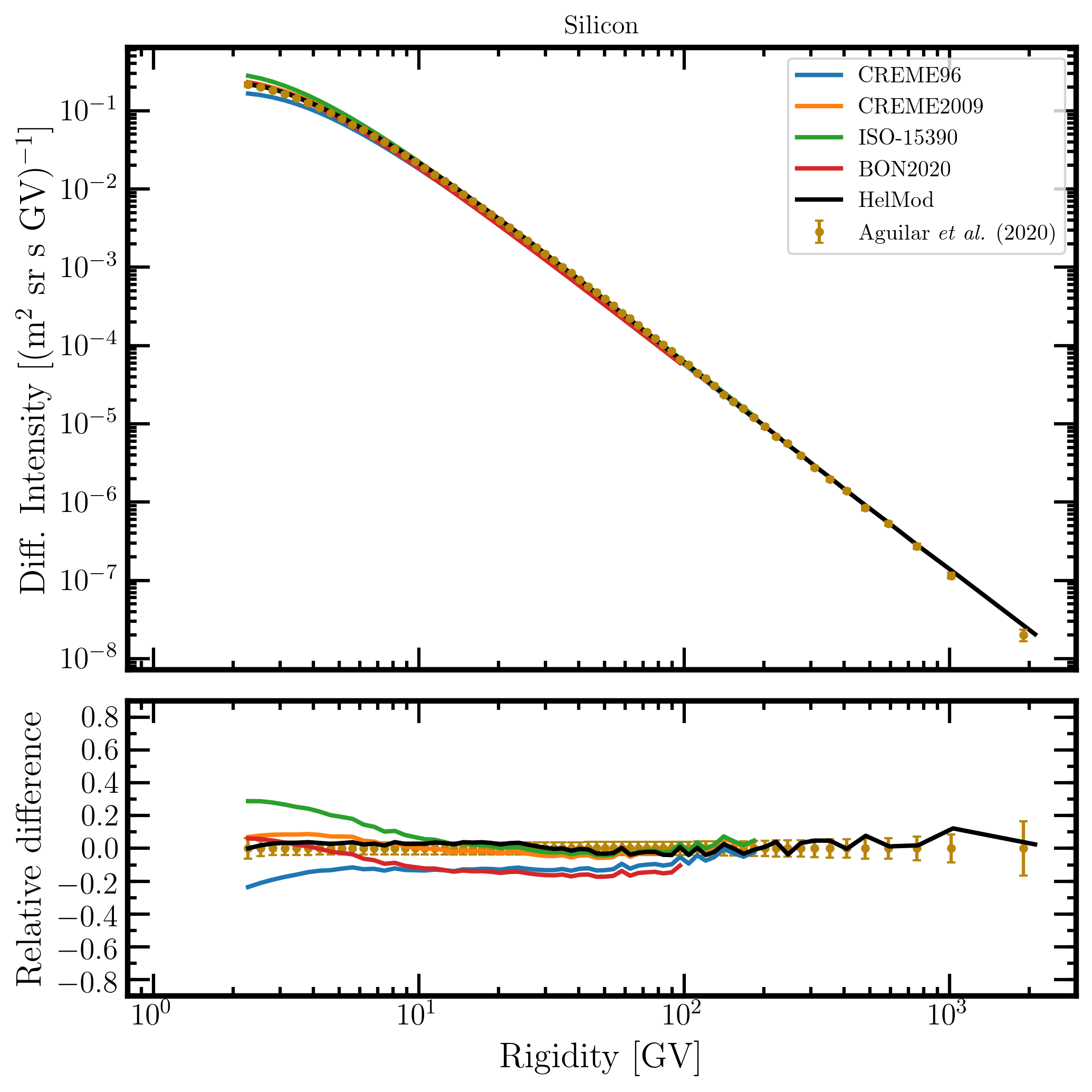
Figure 24. Upper panel: silicon differential intensity in units of [m2 sr s GV]-1 measured by AMS-02 [Aguilar et al. (2020)] (brown points) as a function of rigidity in GV from May 19, 2011, to November 26, 2018, and silicon differential intensities - calculated at 1AU during the same period - for the presently investigated modulation models: CREME96 (blue curve), CREME2009 (orange curve), ISO-15390 (green curve), BON2020 (red curve) and HelMod (black curve). Lower panel: relative differences with respect to AMS-02 data calculated using Eq. (1). Adapted from Figure A18 and Figure 2 of Boschini et al. (2022c).
{tab title="Fig. 25. Iron" class="blue" open="true"}
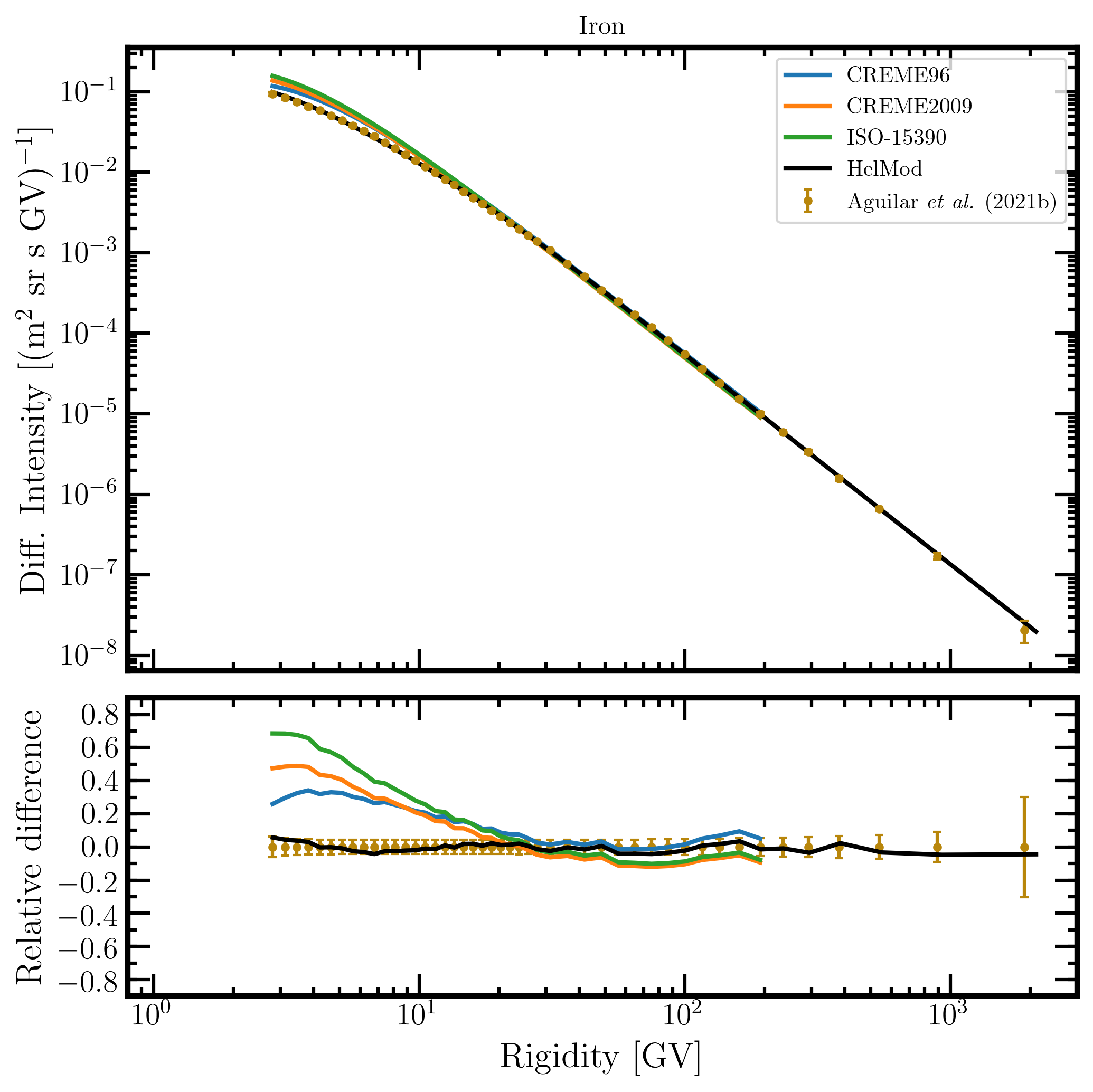
Figure 25. Upper panel: iron differential intensity in units of [m2 sr s GV]-1 measured by AMS-02 [Aguilar et al. (2021b)] (brown points) as a function of rigidity in GV from May 19, 2011, to October 30, 2019, and iron differential intensities - calculated at 1AU during the same period - for the presently investigated modulation models: CREME96 (blue curve), CREME2009 (orange curve), ISO-15390 (green curve), and HelMod (black curve). Lower panel: relative differences with respect to AMS-02 data calculated using Eq. (1). Adapted from Figure A19 and Figure 1 of Boschini et al. (2022c).
{/tabs}
By inspection of Figures 11-25, one can remark that the HelMod model exhibits an overall better agreement with AMS-02 data when compared to the other solar modulation models here presented.
Furthermore, the relative difference of fluences (i.e., the computed integrals of differential intensities over rigidity) evaluated from solar modulation models and that from AMS–02 data is computed by:
 , (2)
, (2)
where Φ(Rmin, Rmax) and ΦAMS-02(Rmin, Rmax) are the fluences of the solar model and that of AMS-02, respectively, in [m2 sr s]-1 in the rigidity interval between Rmin ---the minimum rigidity measured by AMS–02 (i.e., 1 GV for proton, ∼2 GV for other nuclei)--- and Rmax expressed in GV. Most of the considered models do not provide modulated spectra over the full rigidity range covered by AMS–02 experiment (i.e., up to TV). In particular, the BON2020 modulated spectra are provided up to 50 GeV/n, i.e., using Eq. (1) about 50 GV for proton and about 100 GV for the other nuclei.
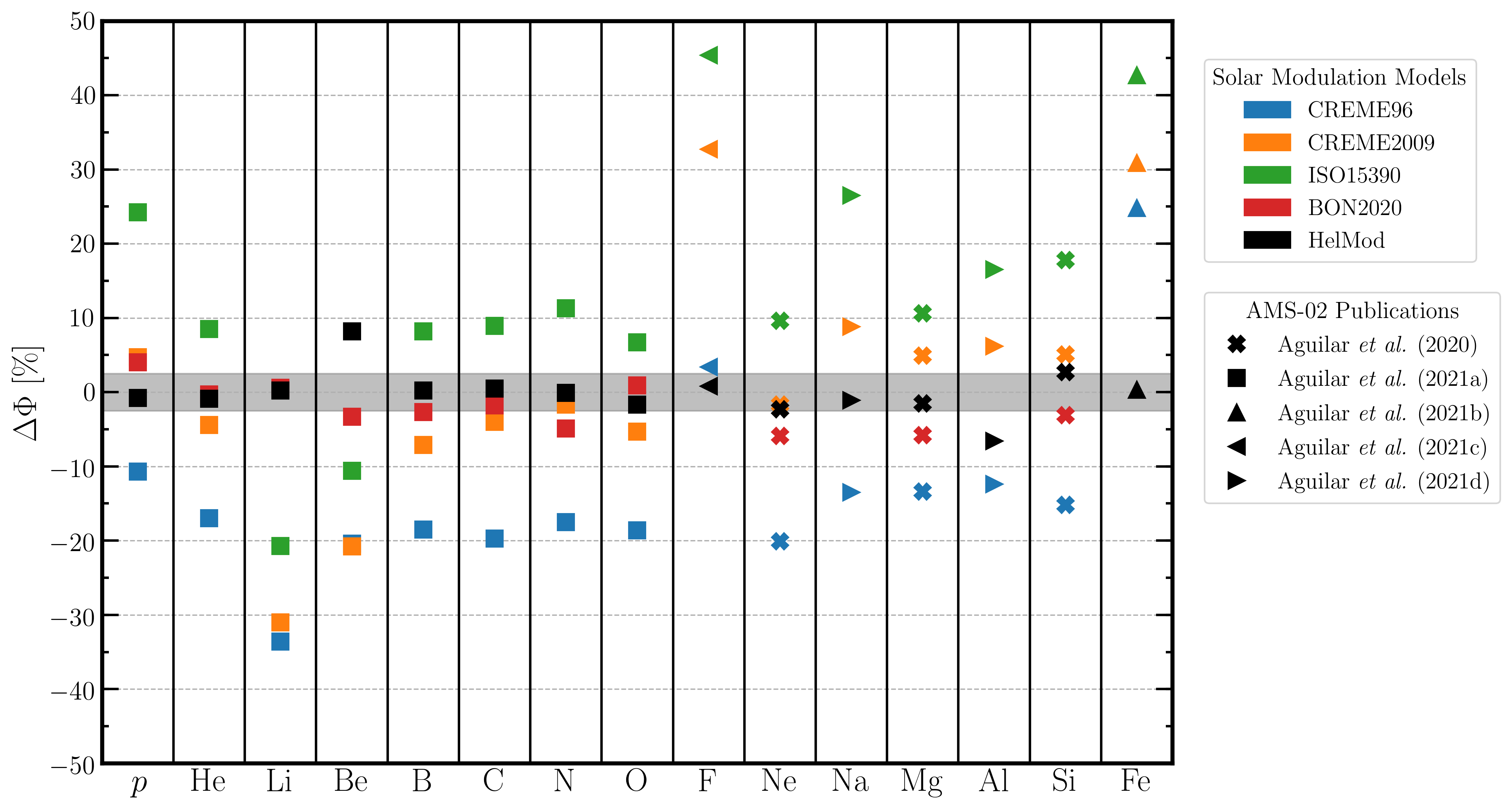
Figure 26. ΔΦ values in percentage (see Eq. 2) for each model and each AMS–02 data set calculated up to Rmax. For the HelMod model, such a quantity was also calculated for the full rigidity range; the so-obtained value is almost overlapping that up to Rmax. The shaded area corresponds to |ΔΦ| < 2.5%. Reproduced from Figure 3 of Boschini et al. (2022c).
By inspection of Fig. 26, one can remark that the HelMod model achieves a good agreement over the full set of experimental data with, typically, ∆Φ within ±2.5%.
A further comparison among solar modulation models and observations was carried out by investigating how the expectations values differ from the experimental ones within the experimental errors, i.e., computing the quantity [Bobik et al. (2012)] (see Figure 27)
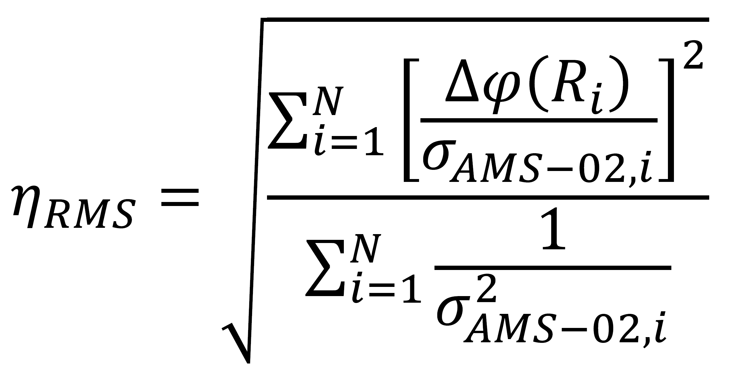 , (3)
, (3)
where σAMS-02,i is the AMS-02 experimental relative error for the i-th data point, and Δφ(Ri) is obtained using Eq. (1).
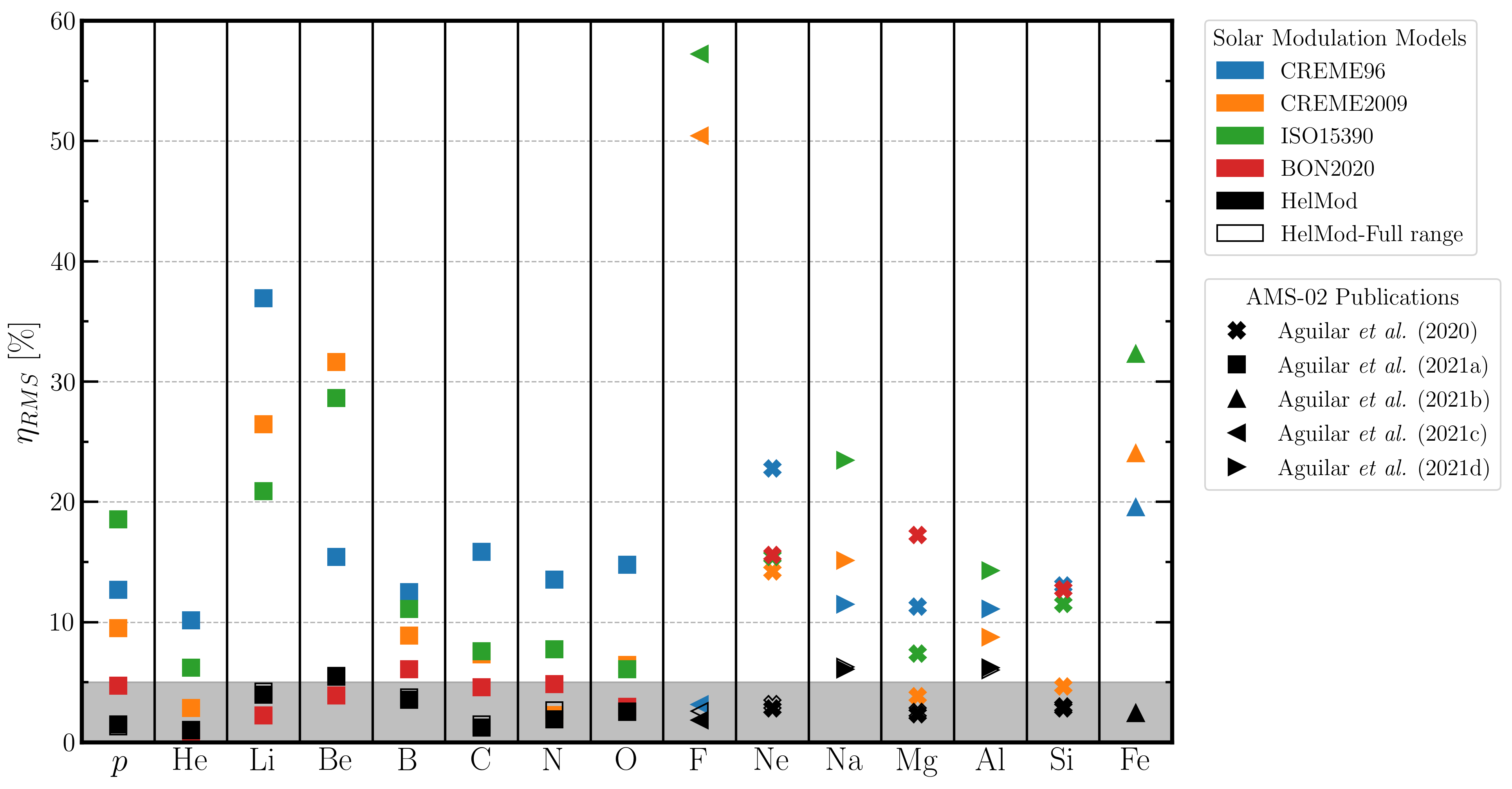
Figure 27. ηRMS values in percentage (see Eq. 3) for each model and each AMS–02 dataset for the incoming particle rigidity up to Rmax. For the HelMod model, such a quantity was also computed for the entire rigidity range available (open markers). The shaded area corresponds to ηRMS < 5%. Reproduced from Figure 4 of Boschini et al. (2022c).
By inspection of Fig. 27, one can remark that the HelMod model again exhibits an overall better agreement with AMS-02 data when compared to the other solar modulation models here investigated with, typically, ηRMS within 5%.
Additional discussions can be found in the published paper by Boschini et al. (2022c).
In addition, the HelMod model is capable of providing the expected differential intensities for GCRs species in any heliospheric position (e.g., see Figure 1, discussions in [Boschini et al. (2019)] and references therein).
Currently, the HelMod code relies on HelMod-4/CUDA, which is a GPU-accelerated method for solving the Parker Equation (e.g., see Della Torre et al., Advantages of GPU-accelerated approach for solving the Parker equation in the heliosphere (2023)). It exploits an NVIDIA GPU farm developed under ASIF program. therein). The code is an evolution of the HelMod-4 code, porting the algorithm to GPU architecture using the CUDA programming language. This approach achieves significant speedup compared to a CPU implementation (e.g., see this webpage). The HelMod-4/CUDA code has been validated by comparing its results with the most precise and updated experimental GCR spectra observed during high and low solar activity periods, both in the inner and outer heliosphere, at the Earth location, and outside the ecliptic plane. The comparison shows that HelMod-4 and HelMod-4/CUDA can be equivalently used to provide solar-modulated spectra with a similar degree of accuracy in reproducing observed data.
Bibliography
[Adriani et al. (2011)] Adriani, O. et al. (2011). Cosmic-Ray Electron Flux Measured by the PAMELA Experiment between 1 and 625 GeV, Phys. Rev. Lett. 106, 201101, doi:10.1103/PhysRevLett.106.201101.
[Adriani et al. (2014)] Adriani, O. et al. (PAMELA Collaboration) (2014), MEASUREMENT OF BORON AND CARBON FLUXES IN COSMIC RAYS WITH THE PAMELA EXPERIMENT, ApJ, 791, 93, doi:10.1088/0004-637X/791/2/93.
[ANSI (2004)] American National Standards Institute, Space environment (natural and artificial) – Galactic cosmic ray model (2004). Tech. Rep. ISO 15390, Washington, D.C. Retrieved from https://www.iso.org/standard/37095.html.
[Aguilar et al. (2014)] Aguilar, M. et al. (AMS Collaboration) (2014). Electron and Positron Fluxes in Primary Cosmic Rays Measured with the Alpha Magnetic Spectrometer on the International Space Station, Phys. Rev. Lett. 113, 121102, doi:10.1103/PhysRevLett.113.121102.
[Aguilar et al. (2015a)] Aguilar, M. et al. (AMS Collaboration) (2015). Precision Measurement of the Proton Flux in Primary Cosmic Rays from Rigidity 1 GV to 1.8 TV with the Alpha Magnetic Spectrometer on the International Space Station, Phys. Rev. Lett. 114, 171103, doi:10.1103/PhysRevLett.114.171103.
[Aguilar et al. (2015b)] Aguilar, M. et al. (AMS Collaboration) (2015). Precision Measurement of the Helium Flux in Primary Cosmic Rays of Rigidities 1.9 GV to 3 TV with the Alpha Magnetic Spectrometer on the International Space Station, Phys. Rev. Lett. 115, 211101, doi:10.1103/PhysRevLett.115.211101.
[Aguilar et al. (2017)] Aguilar, M. et al. (AMS Collaboration) (2017). Observation of the Identical Rigidity Dependence of He, C, and O Cosmic Rays at High Rigidities by the Alpha Magnetic Spectrometer on the International Space Station, Phys. Rev. Lett. 119, 251101, doi:10.1103/PhysRevLett.119.251101.
[Aguilar et al. (2018b)] Aguilar, M. et al. (AMS Collaboration) (2018), Observation of New Properties of Secondary Cosmic Rays Lithium, Beryllium, and Boron by the Alpha Magnetic Spectrometer on the International Space Station, Phys. Rev. Lett. 120, 021101, doi:10.1103/PhysRevLett.120.021101.
[Aguilar et al. (2018c)] Aguilar, M. et al. (AMS Collaboration) (2018), Precision Measurement of Cosmic-Ray Nitrogen and its Primary and Secondary Components with the Alpha Magnetic Spectrometer on the International Space Station, Phys. Rev. Lett.121, 051103, doi:10.1103/PhysRevLett.121.051103.
[Aguilar et al. (2020)] Aguilar, M. et al. (AMS Collaboration) (2020). Properties of Neon, Magnesium, and Silicon Primary Cosmic Rays: Results from the Alpha Magnetic Spectrometer. Phys. Rev. Lett., 124, 211102. doi:10.1103/PhysRevLett.124.211102.
[Aguilar et al. (2021a)] Aguilar, M. et al. (AMS Collaboration) (2021a). The Alpha Magnetic Spectrometer (AMS) on the International Space Station: Part II - Results from the First Seven Years, Physics Reports, 894, 1–116. doi:10.1016/j.physrep.2020.09.003.
[Aguilar et al. (2021b)] Aguilar, M. et al. (AMS Collaboration) (2021b). Properties of Iron Primary Cosmic Rays: Results from the Alpha Magnetic Spectrometer. Phys. Rev. Lett., 126, 041104. doi:10.1103/PhysRevLett.126.041104.
[Aguilar et al. (2021c)] Aguilar, M. et al. (AMS Collaboration) (2021c). Properties of Heavy Secondary Fluorine Cosmic Rays: Results from the Alpha Magnetic Spectrometer. Phys. Rev. Lett., 126, 081102. doi:10.1103/PhysRevLett.126.081102.
[Aguilar et al. (2021d)] Aguilar, M. et al. (AMS Collaboration) (2021d). Properties of a new group of cosmic nuclei: Results from the alpha magnetic spectrometer on sodium, aluminum, and nitrogen. Phys. Rev. Lett., 127, 021101. doi:10.1103/PhysRevLett.127.021101.
[Bobik et al. (2012)] Bobik, P. et al. (2012), Systematic Investigation of Solar Modulation of Galactic Protons for Solar Cycle 23 Using a Monte Carlo Approach with Particle Drift Effects and Latitudinal Dependence, Astrophys. J. 745:132, doi:10.1088/0004-637X/745/2/132.
[Boschini et al. (2017)] Boschini, M. J. et al. (2017). Solution of Heliospheric Propagation: Unveiling the Local Interstellar Spectrum of Cosmic Rays Species, Astrophysical Journal, 840:115, doi:10.3847/1538-4357/aa6e4f.
[Boschini et al. (2018a)] Boschini, M. J. et al. (2018). HelMod In The Works: From Direct Observations To The Local Interstellar Spectrum Of Cosmic-Ray Electrons, Astrophys. J. 854(2):94, doi:10.3847/1538-4357/aaa75e.
[Boschini et al. (2018b)] Boschini, M. J. et al. (2018). Deciphering the Local Interstellar Spectra of Primary Cosmic-Ray Species with HelMod, Astrophys. J. 858(1):61, doi:10.3847/1538-4357/aabc54.
[Boschini et al. (2018c)] M.J. Boschini, S. Della Torre, M. Gervasi, G. La Vacca, P.G. Rancoita, Propagation of cosmic rays in heliosphere: The HelMod model, Advances in Space Res. 62 (2018), 2859-2879, doi:10.1016/j.asr.2017.04.017.
[Boschini et al. (2019)] M.J. Boschini, S. Della Torre, M. Gervasi, G. La Vacca and P.G. Rancoita, The HelMod Model in the Works for Inner and Outer Heliosphere: from AMS to Voyager Probes Observations, Advances in Space Res 64 (2019), 2459-2476, doi:10.1016/j.asr.2019.04.007.
[Boschini et al. (2020a)] Boschini, M. J. et al. (2020a), Deciphering the local interstellar spectra of secondary nuclei with the GALPROP/HelMod framework and a hint for primary lithium in cosmic rays. Astrophys. J., 889(2), 167. doi:10.3847/1538-4357/ab64f1.
[Boschini et al. (2020b)] Boschini, M. J. et al. (2020b). Inference of the local interstellar spectra of cosmic-ray nuclei Z≤28 with the GalProp-HelMod framework. Astrophys. J. Supplement, 250(2), 27. doi:10.3847/1538-4365/aba901.
[Boschini et al. (2021)] Boschini, M. J. et al. (2021) The Discovery of a Low-energy Excess in Cosmic-Ray Iron: Evidence of the Past Supernova Activity in the Local Bubble. The Astrophysical Journal 913(1):5, doi:10.3847/1538-4357/abf11c
[Boschini et al. (2022a)] Boschini, M. J. et al. (2022). A Hint of a Low-energy Excess in Cosmic-Ray Fluorine. The Astrophysical Journal 925(2):108, doi:10.3847/1538-4357/ac313d
[Boschini et al. (2022b)] Boschini, M. J., Della Torre, S., Gervasi, M., La Vacca, G., and Rancoita, P.G., (2022). Forecasting of cosmic rays intensities with HelMod model. Advances in Space Res. (in press) doi:10.1016/j.asr.2022.01.031.
[Boschini et al. (2022c)] Boschini, M. J., Della Torre, S., Gervasi, M., La Vacca, G., and Rancoita, P.G., (2022). The transport of galactic cosmic rays in heliosphere: the HelMod model compared with other commonly employed solar modulation models. Advances in Space Res. (in press) doi:10.1016/j.asr.2022.03.026
[CREME (1996)] Tylka, A. J. et al. (1997). CREME96: A Revision of the Cosmic Ray Effects on Micro-Electronics Code, IEEE Trans. Nucl. Sci., 44, 2150-2160, 1997.; Badhwar, G.D. and O'Neill, P.M. (1996), Galactic cosmic radiation model and its applications, Ad. Sp. Res. 17, 7-17; and also: Badhwar, G.D. and O'Neill, P.M. (1992), An improved model of galactic cosmic radiation for space exploration missions, International Journal of Radiation Applications and Instrumentation. Part D. Nuclear Tracks and Radiation Measurements, Volume 20, Issue 3, 403-410, https://doi.org/10.1016/1359-0189(92)90024-P.
[CREME (2012)] Adams, J.H. et al. (2012). CRÈME: The 2011 Revision of the Cosmic Ray Effects on Micro-Electronics Code, IEEE Tran. Nucl. Scie. 59, 3141 - 3147.
S. Della Torre, G. Cavallotto, D. Besozzi, M. Gervasi, G. La Vacca, M. S. Nobile and P.G. Rancoita (2023), Advantages of GPU-accelerated approach for solving the Parker equation in the heliosphere, POS (ICRC2023) 1290; https://pos.sissa.it/444/1290/pdf
[ECSS (2020)] Space Environment. Technical Report ECSS-EST-10-04C Rev.1 European Cooperation for Space Standardization, ESA. URL: https://ecss.nl/standard/ecss-e-st-10-04c-rev-1-space-environment-15-june-2020/.
[GalProp-HelMod (2016)] GalProp-HelMod (2016). As advertised on the GALPROP website, the HelMod website can be used as a service package to seamlessly calculate the effects of the heliospheric modulation for GALPROP output files. FROM GalProp homepage: "We are pleased to inform the community of the launch of a new service HelMod, which can be used to seamlessly calculate the effects of the heliospheric modulation for GALPROP output file".
[George et al. (2009)] George, J. S. et al. (2009), ELEMENTAL COMPOSITION AND ENERGY SPECTRA OF GALACTIC COSMIC RAYS DURING SOLAR CYCLE 23, ApJ, 698, 1666, doi:10.1088/0004-637X/698/2/1666.
[HelMod (2022)] See [Boschini et al. (2022a)], [Boschini et al. (2022b)], [Boschini et al. (2022c)], [Boschini et al. (2021)], [Boschini et al. (2020a)], [Boschini et al. (2020b)], [Boschini et al. (2019)], [Boschini et al. (2018a)], [Boschini et al. (2018b)], [Boschini et al. (2017)], [Bobik et al. (2012)]; see also: Bobik et al. (2016), On the forward-backward-in-time approach for Monte Carlo solution of Parker's transport equation: One-dimensional case, Journal of Geophysical Research - Space Physics 121(5), 3920–3930, doi:10.1002/2015JA022237.
[Leroy and Rancoita (2016)] C. Leroy and P.G. Rancoita (2016), Principles of Radiation Interaction in Matter and Detection - 4th Edition -, World Scientific. Singapore, ISBN-978-981-4603-18-8 (printed); ISBN.978-981-4603-19-5 (ebook); https://www.worldscientific.com/worldscibooks/10.1142/9167#t=aboutBook; it is also partially accessible via google books.
[Matthiä et al (2013)] Matthiä D., Berger T., Mrigakshi A. I., Reitz G. (2013), A ready-to-use galactic cosmic ray model, Advances in Space Research, Volume 51, Issue 3, Pages 329-338, https://doi.org/10.1016/j.asr.2012.09.022.
K. W. Ogilvie, M. A. Coplan (1995). Solar wind composition, Rev. of Geophysics 33, pages 615-622; https://articles.adsabs.harvard.edu/pdf/1958ApJ...128..664P
[NASA-Voyager (2018)] NASA-Voyager (2018), Online Database, https://voyager.gsfc.nasa.gov/flux.html.
[O’Neill et al. (2015)] O’Neill, P. M., Golge, S., & Slaba, T. C. (2015). Badhwar-O’Neill 2014 Galactic Cosmic Ray Flux Model Description. Technical Report NASA/TP-2015-218569 NASA, USA. URL: https://ntrs.nasa.gov/citations/20150003026.
E.N. Parker (1958). Dynamics of the Interplanetary Gas and Magnetic Fields, Astrophys. J. 128, 664; https://articles.adsabs.harvard.edu/pdf/1958ApJ...128..664P
E.N. Parker (1965). The passage of energetic charged particles through interplanetary space, Planetary and Space Science 13, Pages 9-49; https://doi.org/10.1016/0032-0633(65)90131-5
[Slaba&Whitman (2019)] Slaba, T. C., & Whitman, K. (2019). The Badhwar-O’Neill 2020 Model. Technical Report NASA/TP-2019-220419 NASA, USA. URL: https://ntrs.nasa.gov/citations/20190033460.
L. Svalgaard and Y. Kamide (2013), ASYMMETRIC SOLAR POLAR FIELD REVERSALS, APJ 763:23 (6pp); http://dx.doi.org/10.1088/0004-637X/763/1/23